Timeseries#
In this section of the tutorial, you will learn about the TimeSeries object.
TimeSeries objects hold time-dependent data with their accompanying metadata.
They can be used with multiple one-dimensional arrays which are all associated with a common time axis.
Much like the Map object, the TimeSeries object can handle generic data, but also provides instrument specific data loading and plotting capabilities.
Importantly, TimeSeries allows you to select specific time ranges or combine multiple TimeSeries in a metadata-aware way.
By the end of this tutorial, you will learn how to create a TimeSeries, extract the data and metadata, and easily visualize the TimeSeries. Additionally, you will learn how to truncate a TimeSeries to a specific window in time as well as combine multiple TimeSeries objects.
Note
In this section and in Maps, we will use the sample data included with sunpy.
These data are primarily useful for demonstration purposes or simple debugging.
These files have names like sunpy.data.sample.EVE_TIMESERIES and sunpy.data.sample.GOES_XRS_TIMESERIES and are automatically downloaded to your computer as you need them.
Once downloaded, these sample data files will be paths to their location on your computer.
Creating a TimeSeries#
To create a TimeSeries from some sample GOES XRS data:
>>> import sunpy.timeseries
>>> import sunpy.data.sample

>>> sunpy.data.sample.GOES_XRS_TIMESERIES
PosixPath('.../go1520110607.fits')
>>> my_timeseries = sunpy.timeseries.TimeSeries(sunpy.data.sample.GOES_XRS_TIMESERIES)
In many cases, sunpy will automatically detect the type of the file as well as the instrument associated with it. In this case, we have a FITS file containing an X-ray light curve as observed by the the XRS instrument on the GOES satellite.
Note
Time series data are stored in a variety of file types (e.g. FITS, csv, CDF), and so it is not always possible to detect the source. sunpy ships with a number of known instrumental sources, and can also load CDF files that conform to the Space Physics Guidelines for CDF.
To make sure this has all worked correctly, we can take a quick look at my_timeseries,
>>> my_timeseries
<sunpy.timeseries.sources.goes.XRSTimeSeries object at ...>
SunPy TimeSeries
----------------
Observatory:                 GOES-15
Instrument:          <a href=https://www.swpc.noaa.gov/products/goes-x-ray-flux target="_blank">X-ray Detector</a>
Channel(s):          xrsa<br>xrsb
Start Date:          2011-06-07 00:00:00
End Date:            2011-06-07 23:59:58
Center Date:                 2011-06-07 11:59:58
Resolution:          2.048 s
Samples per Channel:                 42177
Data Range(s):               xrsa   3.64E-06<br>xrsb   2.54E-05
Units:               W / m2
                                       xrsa          xrsb
2011-06-06 23:59:59.961999893  1.000000e-09  1.887100e-07
2011-06-07 00:00:02.008999944  1.000000e-09  1.834600e-07
2011-06-07 00:00:04.058999896  1.000000e-09  1.860900e-07
2011-06-07 00:00:06.104999900  1.000000e-09  1.808400e-07
2011-06-07 00:00:08.151999950  1.000000e-09  1.860900e-07
...                                     ...           ...
2011-06-07 23:59:49.441999912  1.000000e-09  1.624800e-07
2011-06-07 23:59:51.488999844  1.000000e-09  1.624800e-07
2011-06-07 23:59:53.538999915  1.000000e-09  1.598500e-07
2011-06-07 23:59:55.584999919  1.000000e-09  1.624800e-07
2011-06-07 23:59:57.631999850  1.000000e-09  1.598500e-07

[42177 rows x 2 columns]
This should show a table of information taken from the metadata and a preview of your data.
If you are in a Jupyter Notebook, this will show a rich HTML version that includes plots of the data.
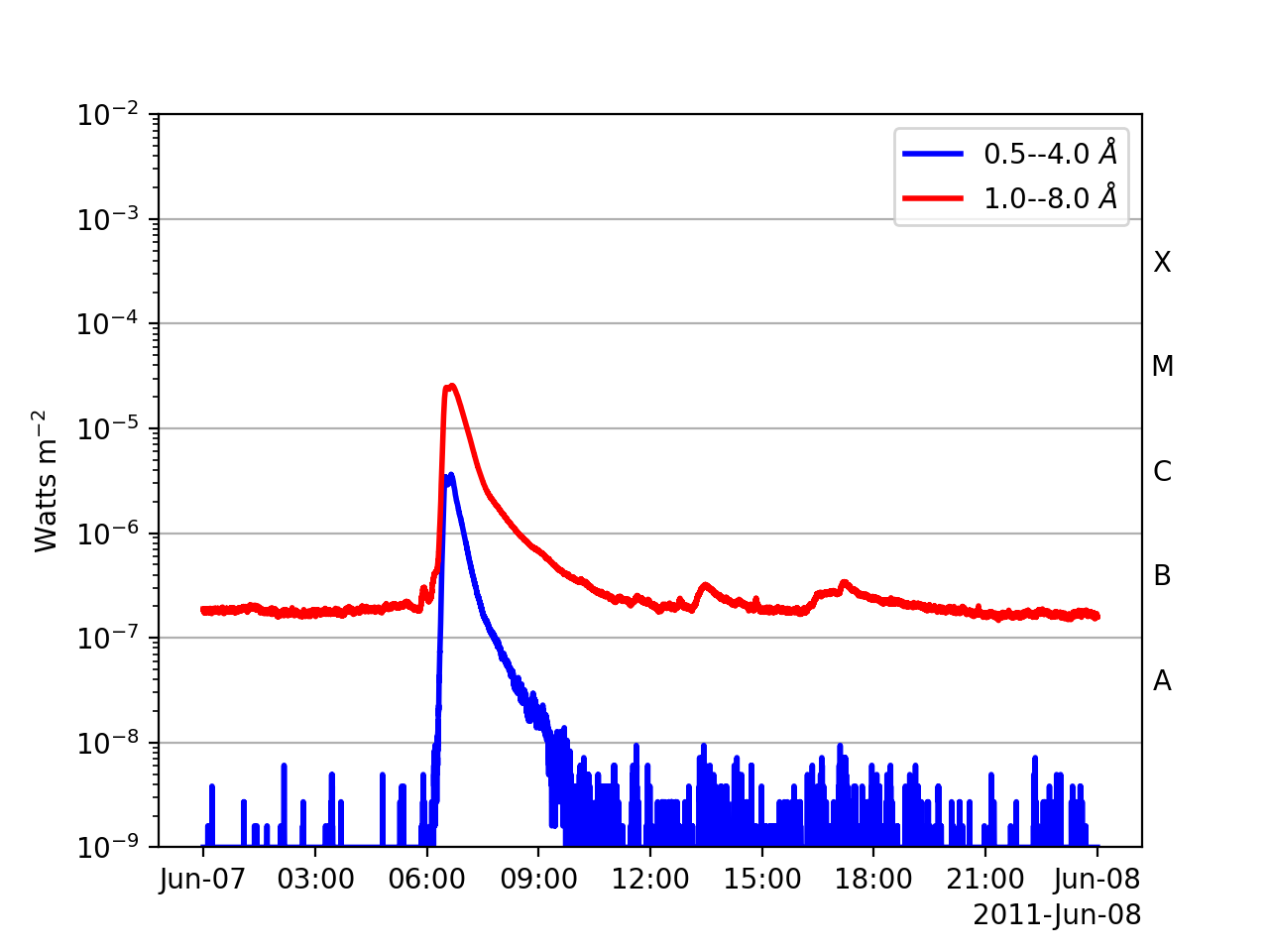
Otherwise, you can use the quicklook() method to see this quick-look plot,
>>> my_timeseries.quicklook()
<sunpy.timeseries.sources.goes.XRSTimeSeries object at 0x744f8c4b16d0>
|

|
||||||||||||||||||||

|
TimeSeries Data#
We can easily check which columns are contained in the TimeSeries,
>>> my_timeseries.columns
['xrsa', 'xrsb']
“xrsa” denotes the short wavelength channel of the XRS data which contains emission between 0.5 and 4 Angstrom.
To pull out the just the data corresponding to this column, we can use the quantity() method:
>>> my_timeseries.quantity('xrsa')
<Quantity [1.e-09, 1.e-09, 1.e-09, ..., 1.e-09, 1.e-09, 1.e-09] W / m2>
Notice that this is a Quantity object which we discussed in Units.
Additionally, the timestamp associated with each point and the time range of the observation are accessible as attributes,
>>> my_timeseries.time
<Time object: scale='utc' format='iso' value=['2011-06-06 23:59:59.962' '2011-06-07 00:00:02.009'
 '2011-06-07 00:00:04.059' ... '2011-06-07 23:59:53.539'
 '2011-06-07 23:59:55.585' '2011-06-07 23:59:57.632']>
>>> my_timeseries.time_range
   <sunpy.time.timerange.TimeRange object at ...>
    Start: 2011-06-06 23:59:59
    End:   2011-06-07 23:59:57
    Center:2011-06-07 11:59:58
    Duration:0.9999730324069096 days or
           23.99935277776583 hours or
           1439.9611666659498 minutes or
           86397.66999995698 seconds
Notice that these return a astropy.time.Time and sunpy.time.TimeRange, both of which we covered in Times.
Inspecting TimeSeries Metadata#
A TimeSeries object also includes metadata associated with that observation. Some of this metadata is exposed via attributes on the TimeSeries. For example, to find out which observatory observed this data,
>>> my_timeseries.observatory
'GOES-15'
Additionally, to find out which instrument this timeseries data came from,
>>> my_timeseries.source
'xrs'
All of the metadata can also be accessed using the meta attribute,
>>> my_timeseries.meta
|-------------------------------------------------------------------------------------------------|
|TimeRange                  | Columns         | Meta                                              |
|-------------------------------------------------------------------------------------------------|
|2011-06-06T23:59:59.961999 | xrsa            | simple: True                                      |
|            to             | xrsb            | bitpix: 8                                         |
|2011-06-07T23:59:57.631999 |                 | naxis: 0                                          |
|                           |                 | extend: True                                      |
|                           |                 | date: 26/06/2012                                  |
|                           |                 | numext: 3                                         |
|                           |                 | telescop: GOES 15                                 |
|                           |                 | instrume: X-ray Detector                          |
|                           |                 | object: Sun                                       |
|                           |                 | origin: SDAC/GSFC                                 |
|                           |                 | ...                                               |
|-------------------------------------------------------------------------------------------------|
Warning
A word of caution: many data sources provide little to no meta data so this variable might be empty. See A Detailed Look at the TimeSeries Metadata for a more detailed explanation of how metadata on TimeSeries objects is handled.
Visualizing TimeSeries#
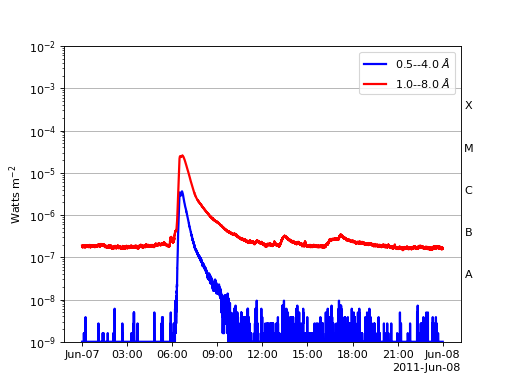
The sunpy TimeSeries object has its own built-in plot methods so that it is easy to quickly view your time series. To create a plot,
import matplotlib.pyplot as plt

fig, ax = plt.subplots()
my_timeseries.plot(axes=ax)
plt.show()
(Source code, png, hires.png, pdf)
Note
For additional examples of building more complex visualization with TimeSeries, see the examples in Time Series.
Adding Columns#
TimeSeries provides the add_column method which will either add a new column or update a current column if the colname is already present.
This can take numpy array or preferably an Astropy Quantity value.
For example:
>>> values = my_timeseries.quantity('xrsa') * 2
>>> my_timeseries = my_timeseries.add_column('xrsa*2', values)
>>> my_timeseries.columns
['xrsa', 'xrsb', 'xrsa*2']
Adding a column is not done in place, but instead returns a new TimeSeries with the new column added.
Note that the values will be converted into the column units if an Astropy Quantity is given.
Caution should be taken when adding a new column because this column won’t have any associated MetaData entry.
Truncating a TimeSeries#
It is often useful to truncate an existing TimeSeries object to retain a specific time range.
This is easily achieved by using the truncate method.
For example, to trim our GOES data into a period of interest use:
>>> from sunpy.time import TimeRange

>>> tr = TimeRange('2012-06-01 05:00', '2012-06-01 06:30')
>>> my_timeseries_trunc = my_timeseries.truncate(tr)
This takes a number of different arguments, such as the start and end dates (as datetime or string objects) or a TimeRange as used above.
Note that the truncated TimeSeries will have a truncated TimeSeriesMetaData object, which may include dropping metadata entries for data totally cut out from the TimeSeries.
If you want to truncate using slice-like values you can, for example taking every 2nd value from 0 to 10000 can be done using:
>>> my_timeseries_trunc = my_timeseries.truncate(0, 100000, 2)
Concatenating TimeSeries#
It’s common to want to combine a number of TimeSeries together into a single TimeSeries.
In the simplest scenario this is to combine data from a single source over several time ranges, for example if you wanted to combine the daily GOES data to get a week or more of constant data in one TimeSeries.
This can be performed using the TimeSeries factory with the concatenate=True keyword argument:
>>> concatenated_timeseries = sunpy.timeseries.TimeSeries(filepath1, filepath2, source='XRS', concatenate=True)
Note, you can list any number of files, or a folder or use a glob to select the input files to be concatenated.
It is possible to concatenate two TimeSeries after creating them using the concatenate method.
For example:
>>> concatenated_timeseries = goes_timeseries_1.concatenate(goes_timeseries_2)
This will result in a TimeSeries identical to if you had created them in one step.
A limitation of the TimeSeries class is that it is not always possible to determine the source observatory or instrument of a given file.
Thus some sources need to be explicitly stated (using the keyword argument) and so, it is not possible to concatenate files from multiple sources.
To do this, you can still use the concatenate method, which will create a new TimeSeries with all the rows and columns of the source and concatenated TimeSeries in one:
>>> eve_ts = sunpy.timeseries.TimeSeries(sunpy.data.sample.EVE_TIMESERIES, source='eve')
>>> concatenated_timeseries = my_timeseries.concatenate(eve_ts)
Note that the more complex TimeSeriesMetaData object now has 2 entries and shows details on both:
>>> concatenated_timeseries.meta
    |-------------------------------------------------------------------------------------------------|
|TimeRange                  | Columns         | Meta                                              |
|-------------------------------------------------------------------------------------------------|
|2011-06-06T23:59:59.961999 | xrsa            | simple: True                                      |
|            to             | xrsb            | bitpix: 8                                         |
|2011-06-07T23:59:57.631999 |                 | naxis: 0                                          |
|                           |                 | extend: True                                      |
|                           |                 | date: 26/06/2012                                  |
|                           |                 | numext: 3                                         |
|                           |                 | telescop: GOES 15                                 |
|                           |                 | instrume: X-ray Detector                          |
|                           |                 | object: Sun                                       |
|                           |                 | origin: SDAC/GSFC                                 |
|                           |                 | ...                                               |
|-------------------------------------------------------------------------------------------------|
|2011-06-07T00:00:00.000000 | XRS-B proxy     | data_list: 20110607_EVE_L0CS_DIODES_1m.txt        |
|            to             | XRS-A proxy     | created: Tue Jun  7 23:59:10 2011 UTC             |
|2011-06-07T23:59:00.000000 | SEM proxy       | origin: SDO/EVE Science Processing and Operations |
|                           | 0.1-7ESPquad    | units: W/m^2 for irradiance, dark is counts/(0.25s|
|                           | 17.1ESP         | source: SDO-EVE ESP and MEGS-P instruments, http:/|
|                           | 25.7ESP         | product: Level 0CS, 1-minute averaged SDO-EVE Sola|
|                           | 30.4ESP         | version: 2.1, code updated 2011-May-12            |
|                           | 36.6ESP         | missing data: -1.00e+00                           |
|                           | darkESP         | hhmm: hour and minute in UT                       |
|                           | 121.6MEGS-P     | xrs-b proxy: a model of the expected XRS-B 0.1-0.8|
|                           | ...             | ...                                               |
|-------------------------------------------------------------------------------------------------|