Visualizing 3D stereoscopic images

How to make an anaglyph 3D image from a stereoscopic observation

We use a stereoscopic observation from July 2023, when the STEREO-A spacecraft and the SDO spacecraft were close in heliographic longitude. See the Wikipedia page on anaglyph 3D, which typically requires red-cyan glasses to visualize.

import copy

import matplotlib.pyplot as plt
from matplotlib.colors import Normalize

import astropy.units as u
from astropy.coordinates import SkyCoord

import sunpy.data.sample
import sunpy.map
from sunpy.coordinates import Helioprojective

Download co-temporal SDO/AIA image STEREO/EUVI images. The EUVI map does not explicitly define their reference radius of the Sun, so we set it to be the same as for the AIA map to silence some informational messages.

aia_map = sunpy.map.Map(sunpy.data.sample.AIA_STEREOSCOPIC_IMAGE)
euvi_map = sunpy.map.Map(sunpy.data.sample.EUVI_STEREOSCOPIC_IMAGE)
euvi_map.meta['rsun_ref'] = aia_map.meta['rsun_ref']

Verify that the angular separation between the two vantage points is a few degrees. If the angular separation much larger, the 3D effect will be bad.

print(euvi_map.observer_coordinate.separation(aia_map.observer_coordinate))

3d43m07.52520019s

Define a convenience function to reproject an input map to an observer in same direction, but at a distance of 1 AU, and then reproject both maps. The purpose is to make the Sun exactly the same size in pixels in both maps.

def reproject_to_1au(in_map):
    header = sunpy.map.make_fitswcs_header(
        (1000, 1000),
        SkyCoord(
            0*u.arcsec, 0*u.arcsec,
            frame='helioprojective',
            obstime=in_map.date,
            observer=in_map.observer_coordinate.realize_frame(
                in_map.observer_coordinate.represent_as('unitspherical') * u.AU
            )
        ),
        scale=(2.2, 2.2)*u.arcsec/u.pixel
    )
    with Helioprojective.assume_spherical_screen(in_map.observer_coordinate):
        return in_map.reproject_to(header)


euvi_map = reproject_to_1au(euvi_map)
aia_map = reproject_to_1au(aia_map)

/home/docs/checkouts/readthedocs.org/user_builds/sunpy/conda/latest/lib/python3.10/site-packages/sunpy/map/mapbase.py:2757: SunpyUserWarning: rsun mismatch detected: EUVI-A 171.0 Angstrom 2023-07-06 00:05:25.rsun_meters=696000000.0 m;  2023-07-06 00:05:25.rsun_meters=695700000.0 m. This might cause unexpected results during reprojection.
  warn_user("rsun mismatch detected: "
/home/docs/checkouts/readthedocs.org/user_builds/sunpy/conda/latest/lib/python3.10/site-packages/sunpy/map/mapbase.py:2757: SunpyUserWarning: rsun mismatch detected: AIA 171.0 Angstrom 2023-07-06 00:05:33.rsun_meters=696000000.0 m;  2023-07-06 00:05:33.rsun_meters=695700000.0 m. This might cause unexpected results during reprojection.
  warn_user("rsun mismatch detected: "

Define linear scaling for the two images so that they look the same. The values here are empirical.

euvi_norm = Normalize(vmin=750, vmax=1e4, clip=True)
aia_norm = Normalize(vmin=0, vmax=2.1e3, clip=True)

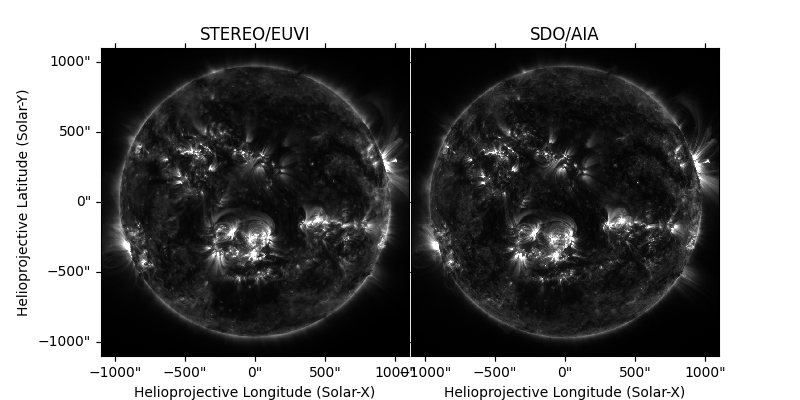
Plot the two maps side by side. Those who are able to see 3D images by defocusing their eyes can see the 3D effect without the later anaglyph image.

fig = plt.figure(figsize=(8, 4))
fig.subplots_adjust(wspace=0)

ax1 = fig.add_subplot(121, projection=euvi_map)
euvi_map.plot(axes=ax1, cmap='gray', norm=euvi_norm)
ax1.grid(False)
ax1.set_title('STEREO/EUVI')

ax2 = fig.add_subplot(122, projection=aia_map)
aia_map.plot(axes=ax2, cmap='gray', norm=aia_norm)
ax2.coords[1].set_ticks_visible(False)
ax2.coords[1].set_ticklabel_visible(False)
ax2.grid(False)
ax2.set_title('SDO/AIA')

Text(0.5, 1.0, 'SDO/AIA')

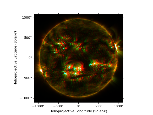
We will make a color anaglyph 3D image by creating two colormaps based on an initial colormap (here, 'sdoaia171'). The left-eye colormap is just the red channel, and the right-eye colormap is just the green and blue channels. Thus, we zero out the appropriate channels in the two colormaps.

cmap_left = copy.deepcopy(plt.get_cmap('sdoaia171'))
cmap_right = copy.deepcopy(cmap_left)

cmap_left._segmentdata['blue'] = [(0, 0, 0), (1, 0, 0)]
cmap_left._segmentdata['green'] = [(0, 0, 0), (1, 0, 0)]
cmap_right._segmentdata['red'] = [(0, 0, 0), (1, 0, 0)]

Finally, we build the anaglyph 3D image. To easily plot in RGB color channels, we will be passing a NxMx3 array to matplotlib’s imshow. That array needs to be manually normalized (to be between 0 and 1) and colorized (mapped into the 3 color channels). The colorizing actually adds a fourth layer for the alpha layer, so we discard that layer.

fig = plt.figure()
ax = fig.add_subplot(projection=aia_map)

euvi_data = euvi_norm(euvi_map.data)
aia_data = aia_norm(aia_map.data)
ax.imshow((cmap_left(euvi_data) + cmap_right(aia_data))[:, :, 0:3], origin='lower')

ax.set_xlabel('Helioprojective Longitude (Solar-X)')
ax.set_ylabel('Helioprojective Latitude (Solar-Y)')

plt.show()