Differential rotation using coordinate frames#
Normally, coordinates refer to a point in inertial space (relative to the barycenter of the solar system).
Transforming to a different observation time does not move the point itself, but if the coordinate frame origin and/or axis change with time, the coordinate representation is updated to account for this change.
In solar physics an example of a frame that changes with time is the HeliographicStonyhurst (HGS) frame.
Its origin moves with the center of the Sun, and its orientation rotates such that the longitude component of Earth is zero at any given time.
A coordinate in a HGS frame of reference transformed to a HGS frame defined a day later will have a different longitude:
>>> import astropy.units as u
>>> from astropy.coordinates import SkyCoord

>>> from sunpy.coordinates import HeliographicStonyhurst

>>> hgs_coord = SkyCoord(0*u.deg, 0*u.deg, radius=1*u.au, frame='heliographic_stonyhurst', obstime="2001-01-01")
>>> new_frame = HeliographicStonyhurst(obstime="2001-01-02")
>>> new_hgs_coord = hgs_coord.transform_to(new_frame)
>>> hgs_coord.lon, new_hgs_coord.lon
(<Longitude 0. deg>, <Longitude -1.01372559 deg>)
but when transformed to an inertial frame of reference we can see that these two coordinates refer to the same point in space:
>>> hgs_coord.transform_to('icrs')
<SkyCoord (ICRS): (ra, dec, distance) in (deg, deg, AU)
    (101.79107615, 26.05004621, 0.99601156)>
>>> new_hgs_coord.transform_to('icrs')
<SkyCoord (ICRS): (ra, dec, distance) in (deg, deg, AU)
    (101.79107615, 26.05004621, 0.99601156)>
To evolve a coordinate in time such that it accounts for the rotational motion of the Sun, one can use the RotatedSunFrame “metaframe” class as described below.
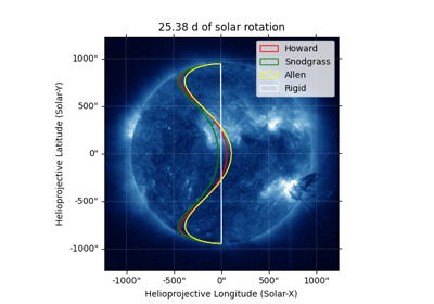
This machinery will take into account the latitude-dependent rotation rate of the solar surface, also known as differential rotation.
Multiple models for differential rotation are supported (see differential_rotate() for details).
Note
RotatedSunFrame is a powerful metaframe, but can be tricky to use correctly.
We recommend users to first check if the simpler propagate_with_solar_surface() context manager is sufficient for their needs.
In addition, one may want to account for the translational motion of the Sun as well, and that can be achieved by also using the context manager transform_with_sun_center() for desired coordinate transformations.
Basics of the RotatedSunFrame class#
The RotatedSunFrame class allows one to specify coordinates in a coordinate frame prior to an amount of solar (differential) rotation being applied.
That is, the coordinate will point to a location in inertial space at some time, but will use a coordinate system at a different time to refer to that point, while accounting for the differential rotation between those two times.
RotatedSunFrame is not itself a coordinate frame, but is instead a “metaframe”.
A new frame class is created on the fly corresponding to each base coordinate frame class.
This tutorial will refer to these new classes as RotatedSun* frames.
Creating coordinates#
RotatedSunFrame requires two inputs: the base coordinate frame and the duration of solar rotation.
The base coordinate frame needs to be fully specified, which means a defined obstime and, if relevant, a defined observer.
Note that the RotatedSun* frame that is created in this example is appropriately named RotatedSunHeliographicStonyhurst:
>>> from sunpy.coordinates import RotatedSunFrame
>>> import sunpy.coordinates.frames as frames

>>> base_frame = frames.HeliographicStonyhurst(obstime="2001-01-01")
>>> rs_hgs = RotatedSunFrame(base=base_frame, duration=1*u.day)
>>> rs_hgs
<RotatedSunHeliographicStonyhurst Frame (base=<HeliographicStonyhurst Frame (obstime=2001-01-01T00:00:00.000, rsun=695700.0 km)>, duration=1.0 d, rotation_model=howard)>
Once a RotatedSun* frame is created, it can be used in the same manner as other frames.
Here, we create a SkyCoord using the RotatedSun* frame:
>>> rotated_coord = SkyCoord(0*u.deg, 0*u.deg, frame=rs_hgs)
>>> rotated_coord
<SkyCoord (RotatedSunHeliographicStonyhurst: base=<HeliographicStonyhurst Frame (obstime=2001-01-01T00:00:00.000, rsun=695700.0 km)>, duration=1.0 d, rotation_model=howard): (lon, lat) in deg
    (0., 0.)>
Transforming this into the original heliographic Stonyhurst frame, we can see that the longitude is equal to the original zero degrees, plus an extra offset to account for one day of differential rotation:
>>> rotated_coord.transform_to(base_frame).lon
<Longitude 14.32632838 deg>
Instead of explicitly specifying the duration of solar rotation, one can use the keyword argument rotated_time.
The duration will be automatically calculated from the difference between rotated_time and the obstime value of the base coordinate frame.
Here, we also include coordinate data in the supplied base coordinate frame:
>>> rs_hgc = RotatedSunFrame(base=frames.HeliographicCarrington(10*u.deg, 20*u.deg, observer="earth",
...                                                        obstime="2020-03-04 00:00"),
...                          rotated_time="2020-03-06 12:00")
>>> rs_hgc
<RotatedSunHeliographicCarrington Coordinate (base=<HeliographicCarrington Frame (obstime=2020-03-04T00:00:00.000, rsun=695700.0 km, observer=<HeliographicStonyhurst Coordinate for 'earth'>)>, duration=2.5 d, rotation_model=howard): (lon, lat) in deg
    (10., 20.)>
A RotatedSun* frame containing coordinate data can be supplied to SkyCoord as normal:
>>> SkyCoord(rs_hgc)
<SkyCoord (RotatedSunHeliographicCarrington: base=<HeliographicCarrington Frame (obstime=2020-03-04T00:00:00.000, rsun=695700.0 km, observer=<HeliographicStonyhurst Coordinate for 'earth'>)>, duration=2.5 d, rotation_model=howard): (lon, lat) in deg
    (10., 20.)>
The above examples used the default differential-rotation model, but any of the models available through sunpy.physics.differential_rotation.differential_rotate() are selectable.
For example, instead of the default (“howard”), one can specify “allen” using the keyword argument rotation_model.
Note the slight difference in the “real” longitude compared to the output above:
>>> allen = RotatedSunFrame(base=frames.HeliographicCarrington(10*u.deg, 20*u.deg, observer="earth",
...                                                               obstime="2020-03-04 00:00"),
...                            rotated_time="2020-03-06 12:00", rotation_model="allen")
>>> allen.transform_to(allen.base)
<HeliographicCarrington Coordinate (obstime=2020-03-04T00:00:00.000, rsun=695700.0 km, observer=<HeliographicStonyhurst Coordinate for 'earth'>): (lon, lat, radius) in (deg, deg, km)
    (45.22266666, 20., 695700.)>
Transforming coordinate arrays#
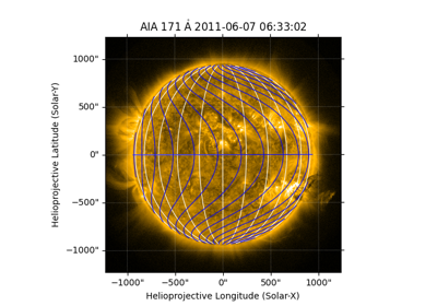
For another transformation example, we define a meridian with a Carrington longitude of 100 degrees, plus 1 day of differential rotation.
Again, the coordinates are already differentially rotated in inertial space; the RotatedSun* frame allows one to represent the coordinates in a frame prior to the differential rotation:
>>> meridian = RotatedSunFrame([100]*11*u.deg, range(-75, 90, 15)*u.deg,
...                            base=frames.HeliographicCarrington(observer="earth", obstime="2001-01-01"),
...                            duration=1*u.day)
>>> meridian
<RotatedSunHeliographicCarrington Coordinate (base=<HeliographicCarrington Frame (obstime=2001-01-01T00:00:00.000, rsun=695700.0 km, observer=<HeliographicStonyhurst Coordinate for 'earth'>)>, duration=1.0 d, rotation_model=howard): (lon, lat) in deg
    [(100., -75.), (100., -60.), (100., -45.), (100., -30.), (100., -15.),
    (100.,   0.), (100.,  15.), (100.,  30.), (100.,  45.), (100.,  60.),
    (100.,  75.)]>
An easy way to “see” the differential rotation is to transform the coordinates to the base coordinate frame. Note that the points closer to the equator (latitude of 0 degrees) have evolved farther in longitude than the points at high latitudes:
>>> meridian.transform_to(meridian.base)
<HeliographicCarrington Coordinate (obstime=2001-01-01T00:00:00.000, rsun=695700.0 km, observer=<HeliographicStonyhurst Coordinate for 'earth'>): (lon, lat, radius) in (deg, deg, km)
    [(110.755047, -75., 695700.), (111.706972, -60., 695700.),
    (112.809044, -45., 695700.), (113.682163, -30., 695700.),
    (114.17618 , -15., 695700.), (114.326328,   0., 695700.),
    (114.17618 ,  15., 695700.), (113.682163,  30., 695700.),
    (112.809044,  45., 695700.), (111.706972,  60., 695700.),
    (110.755047,  75., 695700.)]>
In the specific case of HeliographicCarrington, this frame rotates with the Sun, but in a non-differential manner.
The Carrington longitude approximately follows the rotation of the Sun.
One can transform to the coordinate frame of 1 day in the future to see the difference between Carrington rotation and differential rotation.
Note that equator rotates slightly faster than the Carrington rotation rate (its longitude is now greater than 100 degrees), but most latitudes rotate slower than the Carrington rotation rate:
>>> meridian.transform_to(frames.HeliographicCarrington(observer="earth", obstime="2001-01-02"))
<HeliographicCarrington Coordinate (obstime=2001-01-02T00:00:00.000, rsun=695700.0 km, observer=<HeliographicStonyhurst Coordinate for 'earth'>): (lon, lat, radius) in (deg, deg, km)
    [( 96.71777552, -75.1035280, 695509.61226612),
    ( 97.60193088, -60.0954217, 695194.47689542),
    ( 98.68350999, -45.0808511, 694918.44538999),
    ( 99.54760854, -30.0611014, 694697.75301952),
    (100.03737064, -15.0375281, 694544.31380180),
    (100.18622957, -0.01157236, 694467.21969767),
    (100.03737064,  15.0151761, 694471.58239044),
    ( 99.54760854,  30.0410725, 694557.27090716),
    ( 98.68350999,  45.0645144, 694719.82847332),
    ( 97.60193088,  60.0838908, 694951.31065278),
    ( 96.71777552,  75.0975847, 695238.51302901)]>
Be aware that transformations with a change in obstime will also contend with a translation of the center of the Sun.
Note that the radius component above is no longer precisely on the surface of the Sun.
For precise transformations of solar features, one should also use the context manager transform_with_sun_center() to account for the translational motion of the Sun.
Using the context manager, the radius component stays as the solar radius as desired:
>>> from sunpy.coordinates import transform_with_sun_center

>>> with transform_with_sun_center():
...     print(meridian.transform_to(frames.HeliographicCarrington(observer="earth", obstime="2001-01-02")))
<HeliographicCarrington Coordinate (obstime=2001-01-02T00:00:00.000, rsun=695700.0 km, observer=<HeliographicStonyhurst Coordinate for 'earth'>): (lon, lat, radius) in (deg, deg, km)
    [( 96.570646, -75., 695700.), ( 97.52257 , -60., 695700.),
    ( 98.624643, -45., 695700.), ( 99.497762, -30., 695700.),
    ( 99.991779, -15., 695700.), (100.141927,   0., 695700.),
    ( 99.991779,  15., 695700.), ( 99.497762,  30., 695700.),
    ( 98.624643,  45., 695700.), ( 97.52257 ,  60., 695700.),
    ( 96.570646,  75., 695700.)]>
Transforming multiple durations of rotation#
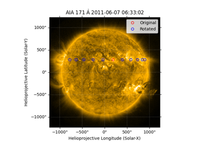
Another common use case for differential rotation is to track a solar feature over a sequence of time steps.
Let’s track an active region that starts at Helioprojective coordinates (-123 arcsec, 456 arcsec), as seen from Earth, and we will look both backwards and forwards in time.
When duration is an array, the base coordinate will be automatically upgraded to an array if it is a scalar.
We specify a range of durations from -5 days to +5 days, stepping at 1-day increments:
>>> durations = range(-5, 6, 1)*u.day
>>> ar_start = frames.Helioprojective(-123*u.arcsec, 456*u.arcsec,
...                              obstime="2001-01-01", observer="earth")
>>> ar = RotatedSunFrame(base=ar_start, duration=durations)
>>> ar
<RotatedSunHelioprojective Coordinate (base=<Helioprojective Frame (obstime=2001-01-01T00:00:00.000, rsun=695700.0 km, observer=<HeliographicStonyhurst Coordinate for 'earth'>)>, duration=[-5. -4. -3. -2. -1.  0.  1.  2.  3.  4.  5.] d, rotation_model=howard): (Tx, Ty) in arcsec
    [(-123., 456.), (-123., 456.), (-123., 456.), (-123., 456.),
    (-123., 456.), (-123., 456.), (-123., 456.), (-123., 456.),
    (-123., 456.), (-123., 456.), (-123., 456.)]>
Let’s convert to the base coordinate frame to reveal the motion of the active region over time:
>>> ar.transform_to(ar.base)
<Helioprojective Coordinate (obstime=2001-01-01T00:00:00.000, rsun=695700.0 km, observer=<HeliographicStonyhurst Coordinate for 'earth'>): (Tx, Ty, distance) in (arcsec, arcsec, AU)
    [(-865.549563, 418.102848, 0.982512),
    (-794.67361 , 429.259359, 0.981549),
    (-676.999492, 439.158483, 0.980695),
    (-519.354795, 447.212391, 0.980001),
    (-330.98304 , 452.940564, 0.979507),
    (-123.      , 456.      , 0.979244),
    (  92.27676 , 456.207078, 0.979226),
    ( 302.081349, 453.54936 , 0.979455),
    ( 493.984308, 448.186389, 0.979917),
    ( 656.653862, 440.439434, 0.980585),
    ( 780.541211, 430.770974, 0.981419)]>
Be aware that these coordinates are represented in the Helioprojective coordinates as seen from Earth at the base time.
Since the Earth moves in its orbit around the Sun, one may be more interested in representing these coordinates as they would been seen by an Earth observer at each time step.
Since the destination frame of the transformation will now have arrays for obstime and observer, one actually has to construct the initial coordinate with an array for obstime (and observer) due to a limitation in Astropy.
Note that the active region moves slightly slower across the disk of the Sun because the Earth orbits in the same direction as the Sun rotates, thus reducing the apparent rotation of the Sun:
>>> ar_start_array = frames.Helioprojective([-123]*len(durations)*u.arcsec,
...                                    [456]*len(durations)*u.arcsec,
...                                    obstime=["2001-01-01"]*len(durations), observer="earth")
>>> ar_array = RotatedSunFrame(base=ar_start_array, duration=durations)
>>> earth_hpc = frames.Helioprojective(obstime=ar_array.rotated_time, observer="earth")
>>> ar_array.transform_to(earth_hpc)
<Helioprojective Coordinate (obstime=['2000-12-27 00:00:00.000' '2000-12-28 00:00:00.000'
'2000-12-29 00:00:00.000' '2000-12-30 00:00:00.000'
'2000-12-31 00:00:00.000' '2001-01-01 00:00:00.000'
'2001-01-02 00:00:00.000' '2001-01-03 00:00:00.000'
'2001-01-04 00:00:00.000' '2001-01-05 00:00:00.000'
'2001-01-06 00:00:00.000'], rsun=695700.0 km, observer=<HeliographicStonyhurst Coordinate for 'earth'>): (Tx, Ty, distance) in (arcsec, arcsec, AU)
    [(-853.35712 , 420.401517, 0.982294),
    (-771.20926 , 429.298481, 0.981392),
    (-650.31062 , 437.85932 , 0.980601),
    (-496.634378, 445.519914, 0.97996 ),
    (-317.863549, 451.731964, 0.9795  ),
    (-123.      , 456.      , 0.979244),
    (  78.103714, 457.916782, 0.979203),
    ( 275.263157, 457.194475, 0.97938 ),
    ( 458.500759, 453.689226, 0.979764),
    ( 618.572111, 447.417202, 0.980336),
    ( 747.448484, 438.560811, 0.981067)]>
Transforming into RotatedSun frames#
So far, all of the examples show transformations with the RotatedSun* frame as the starting frame.
The RotatedSun* frame can also be the destination frame, which can be more intuitive in some situations and even necessary in some others (due to API limitations).
Let’s use a coordinate from earlier, which represents the coordinate in a “real” coordinate frame:
>>> coord = rs_hgc.transform_to(rs_hgc.base)
>>> coord
<HeliographicCarrington Coordinate (obstime=2020-03-04T00:00:00.000, rsun=695700.0 km, observer=<HeliographicStonyhurst Coordinate for 'earth'>): (lon, lat, radius) in (deg, deg, km)
    (45.13354448, 20., 695700.)>
If we create a RotatedSun* frame for a different base time, we can represent that same point using coordinates prior to differential rotation:
>>> rs_frame = RotatedSunFrame(base=frames.HeliographicCarrington(observer="earth",
...                                                          obstime=coord.obstime),
...                            rotated_time="2020-03-06 12:00")
>>> rs_frame
<RotatedSunHeliographicCarrington Frame (base=<HeliographicCarrington Frame (obstime=2020-03-04T00:00:00.000, rsun=695700.0 km, observer=<HeliographicStonyhurst Coordinate for 'earth'>)>, duration=2.5 d, rotation_model=howard)>

>>> new_coord = coord.transform_to(rs_frame)
>>> new_coord
<RotatedSunHeliographicCarrington Coordinate (base=<HeliographicCarrington Frame (obstime=2020-03-04T00:00:00.000, rsun=695700.0 km, observer=<HeliographicStonyhurst Coordinate for 'earth'>)>, duration=2.5 d, rotation_model=howard): (lon, lat, radius) in (deg, deg, km)
    (10., 20., 695700.)>
There coordinates are stored in the RotatedSun* frame, but it can be useful to “pop off” this extra layer and retain only the coordinate representation in the base coordinate frame.
There is a convenience method called as_base() to do exactly that.
Be aware the resulting coordinate does not point to the same location in inertial space, despite the superficial similarity.
Essentially, the component values have been copied from one coordinate frame to a different coordinate frame, and thus this is not merely a transformation between coordinate frames:
>>> new_coord.as_base()
<HeliographicCarrington Coordinate (obstime=2020-03-04T00:00:00.000, rsun=695700.0 km, observer=<HeliographicStonyhurst Coordinate for 'earth'>): (lon, lat, radius) in (deg, deg, km)
    (10., 20., 695700.)>
Example uses of RotatedSunFrame#
Here are the examples in our gallery that use RotatedSunFrame: