Auto-Aligning AIA and HMI Data During Plotting

This example shows how a map is autoaligned when it is plotted on a different reference frame.

See Aligning AIA and HMI Data with Reproject for an alternate approach to image alignment, where one of the maps is modified prior to plotting, and thus is available for purposes other than plotting.

import matplotlib.pyplot as plt

import astropy.units as u

import sunpy.data.sample
import sunpy.map

We use the AIA image and HMI image from the sample data. For the HMI map, we use the special HMI color map, which expects the plotted range to be -1500 to 1500.

map_aia = sunpy.map.Map(sunpy.data.sample.AIA_171_IMAGE)
map_hmi = sunpy.map.Map(sunpy.data.sample.HMI_LOS_IMAGE)
map_hmi.plot_settings['cmap'] = "hmimag"
map_hmi.plot_settings['norm'] = plt.Normalize(-1500, 1500)

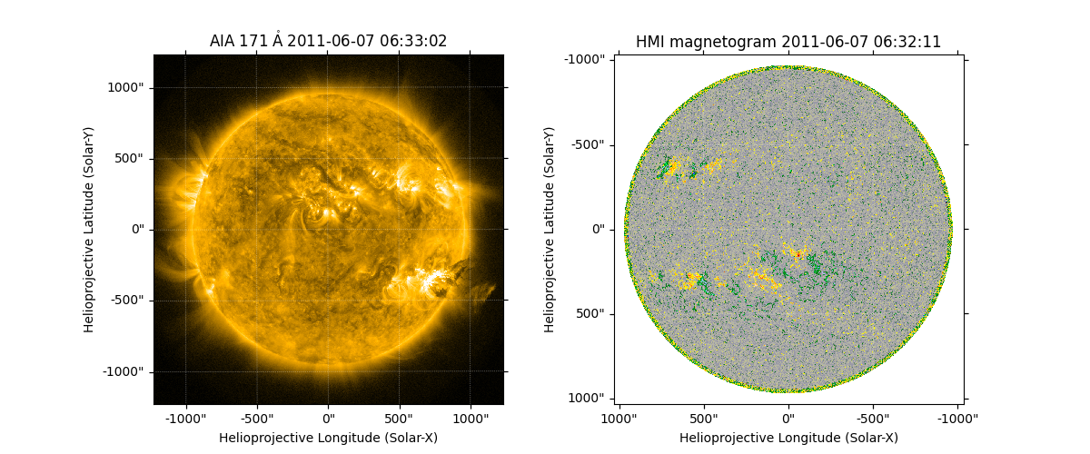
Plot both images side by side. Note by the tick labels that the HMI image is oriented “upside down” relative to the AIA image.

fig = plt.figure(figsize=(12, 5))
ax1 = fig.add_subplot(121, projection=map_aia)
map_aia.plot(axes=ax1, clip_interval=(1, 99.9)*u.percent)
ax2 = fig.add_subplot(122, projection=map_hmi)
map_hmi.plot(axes=ax2)

<matplotlib.image.AxesImage object at 0x7964c143c190>

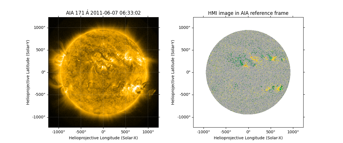
Now let us intentionally set the projection for the right panel to be map_aia instead of map_hmi. This time, plotting the HMI image onto axes defined by the AIA reference frame will trigger “autoalignment” functionality where each map pixel is individually drawn. The HMI image now has the same orientation as the AIA image.

Note that off-disk HMI data are not retained by default because an additional assumption is required to define the location of the HMI emission in 3D space. We can use SphericalScreen to retain the off-disk HMI data. See Reprojecting Using a Spherical Screen for more reference.

fig = plt.figure(figsize=(12, 5))
ax1 = fig.add_subplot(121, projection=map_aia)
map_aia.plot(axes=ax1, clip_interval=(1, 99.9)*u.percent)
ax2 = fig.add_subplot(122, projection=map_aia)
map_hmi.plot(axes=ax2, title='HMI image in AIA reference frame')

INFO: Using mesh-based autoalignment [sunpy.map.mapbase]

<matplotlib.collections.QuadMesh object at 0x7964c22a5090>

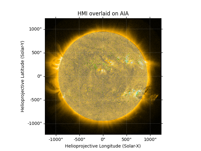
We can directly plot them over one another, by setting the transparency of the HMI plot.

fig = plt.figure()
ax1 = fig.add_subplot(projection=map_aia)
map_aia.plot(axes=ax1, clip_interval=(1, 99.9)*u.percent)
map_hmi.plot(axes=ax1, alpha=0.5)
ax1.set_title('HMI overlaid on AIA')

plt.show()

INFO: Using mesh-based autoalignment [sunpy.map.mapbase]