Note
Go to the end to download the full example code.
Reprojecting Images to Different Observers#
This example demonstrates how you can reproject images to the view from different observers. We use data from these two instruments:
AIA on SDO, which is in orbit around Earth
EUVI on STEREO A, which is in orbit around the Sun away from the Earth
You will need reproject v0.6 or higher installed.
import matplotlib.pyplot as plt

import astropy.units as u
from astropy.coordinates import SkyCoord

import sunpy.map
from sunpy.coordinates import get_body_heliographic_stonyhurst
from sunpy.data.sample import AIA_193_JUN2012, STEREO_A_195_JUN2012
In this example we are going to make a lot of side by side figures, so let’s change the default figure size.
plt.rcParams['figure.figsize'] = (16, 8)
Create a map for each image, after making sure to sort by the appropriate name attribute (i.e., “AIA” and “EUVI”) so that the order is reliable.
map_list = sunpy.map.Map([AIA_193_JUN2012, STEREO_A_195_JUN2012])
map_list.sort(key=lambda m: m.detector)
map_aia, map_euvi = map_list

# We downsample these maps to reduce memory consumption, but you can
# comment this out.
out_shape = (512, 512)
map_aia = map_aia.resample(out_shape * u.pix)
map_euvi = map_euvi.resample(out_shape * u.pix)
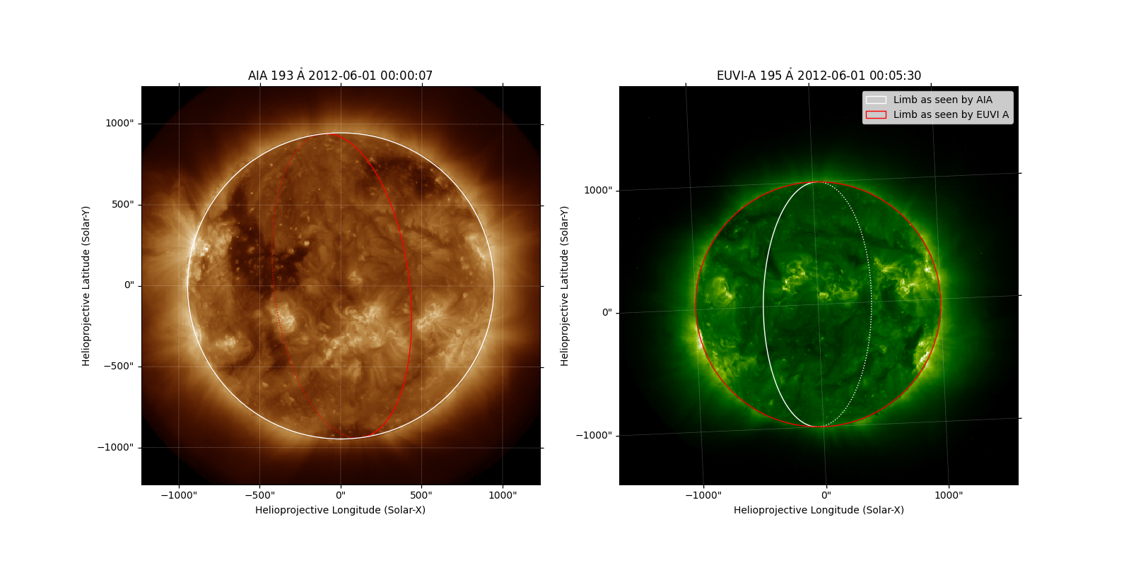
Plot the two maps, with the solar limb as seen by each observatory overlaid on both plots.
fig = plt.figure()

ax1 = fig.add_subplot(121, projection=map_aia)
map_aia.plot(axes=ax1)
map_aia.draw_limb(axes=ax1, color='white')
map_euvi.draw_limb(axes=ax1, color='red')

ax2 = fig.add_subplot(122, projection=map_euvi)
map_euvi.plot(axes=ax2)
limb_aia = map_aia.draw_limb(axes=ax2, color='white')
limb_euvi = map_euvi.draw_limb(axes=ax2, color='red')

plt.legend([limb_aia[0], limb_euvi[0]],
           ['Limb as seen by AIA', 'Limb as seen by EUVI A'])
<matplotlib.legend.Legend object at 0x744fa4a696d0>
Data providers can set the radius at which emission in the map is assumed to have come from. Most maps use a default value for photospheric radius (including EUVI maps), but some maps (including AIA maps) are set to a slightly different value. A mismatch in solar radius means a reprojection will not work correctly on pixels near the limb. This can be prevented by modifying the values for rsun on one map to match the other.
map_euvi.meta['rsun_ref'] = map_aia.meta['rsun_ref']
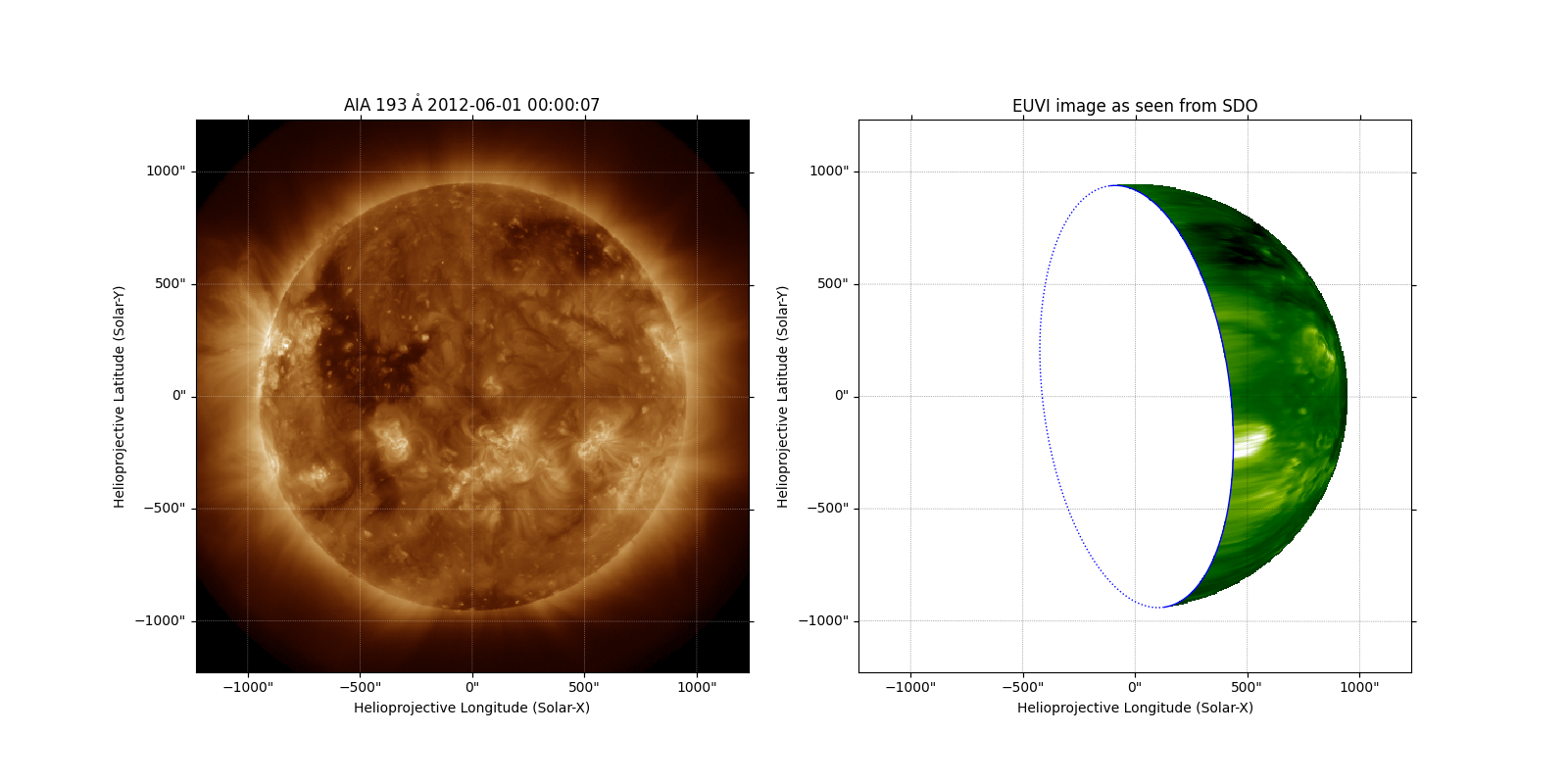
We can reproject the EUVI map to the AIA observer wcs using
reproject_to(). This method defaults to using
the fast reproject.reproject_interp() algorithm, but a different
algorithm can be specified (e.g., reproject.reproject_adaptive()).
outmap = map_euvi.reproject_to(map_aia.wcs)
We can now plot the STEREO/EUVI image as seen from the position of SDO, next to the AIA image.
fig = plt.figure()
ax1 = fig.add_subplot(121, projection=map_aia)
map_aia.plot(axes=ax1)
ax2 = fig.add_subplot(122, projection=outmap)
outmap.plot(axes=ax2, title='EUVI image as seen from SDO')
map_euvi.draw_limb(color='blue')

# Set the HPC grid color to black as the background is white
ax2.grid(color='k')
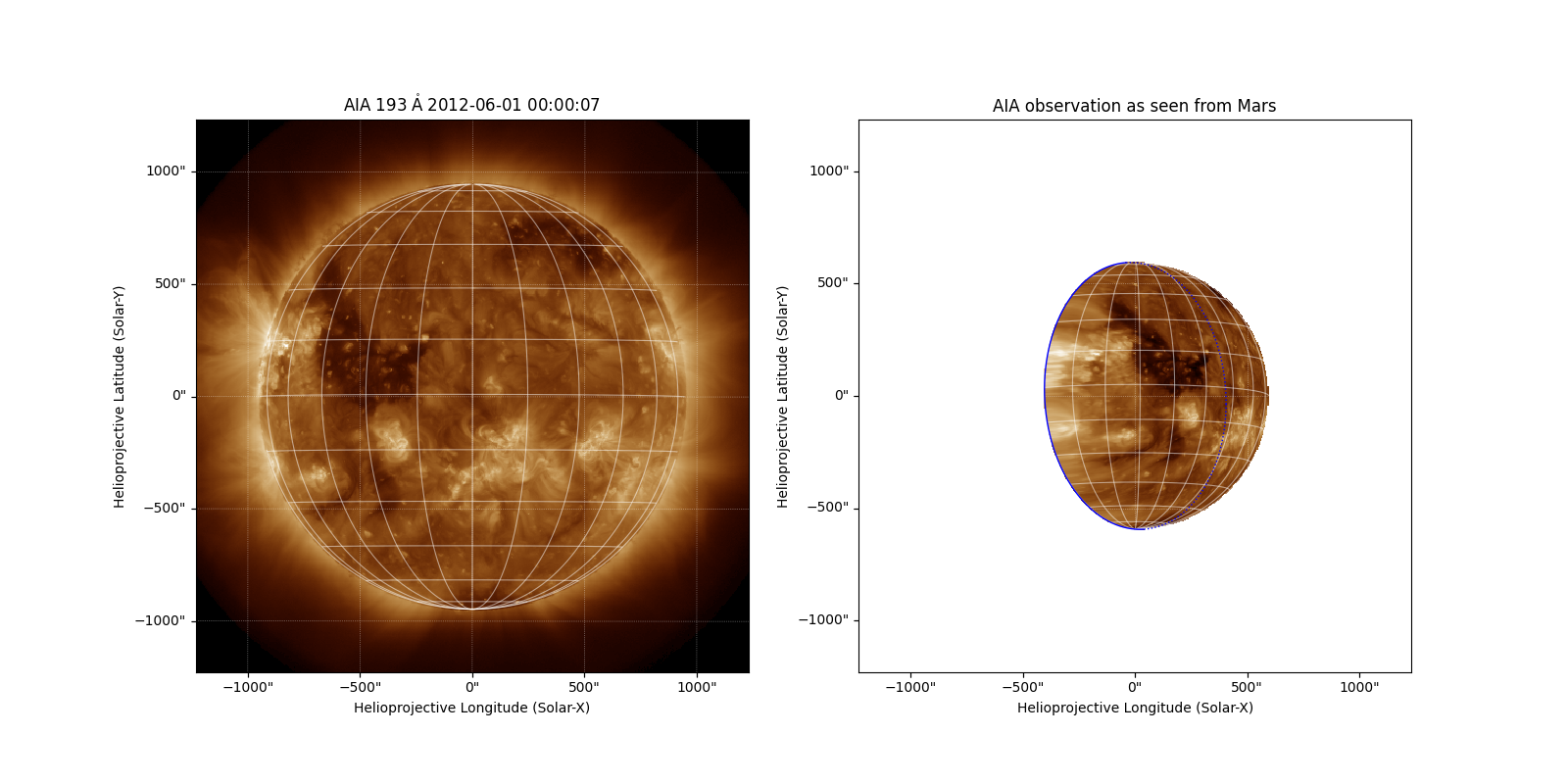
AIA as Seen from Mars#
The new observer coordinate doesn’t have to be associated with an existing Map. sunpy provides a function which can get the location coordinate for any known body. In this example, we use Mars.
mars = get_body_heliographic_stonyhurst('mars', map_aia.date)
Without a target Map wcs, we can generate our own for an arbitrary observer.
First, we need an appropriate reference coordinate. This will be similar to
the one contained in map_aia, except with the observer placed at Mars.
mars_ref_coord = SkyCoord(0*u.arcsec, 0*u.arcsec,
                          obstime=map_aia.reference_coordinate.obstime,
                          observer=mars,
                          rsun=map_aia.reference_coordinate.rsun,
                          frame="helioprojective")
We now need to construct our output WCS; we build a custom header using
sunpy.map.header_helper.make_fitswcs_header() using the map_aia
properties and our new, mars-based reference coordinate.
mars_header = sunpy.map.make_fitswcs_header(
    out_shape,
    mars_ref_coord,
    scale=u.Quantity(map_aia.scale),
    instrument="AIA",
    wavelength=map_aia.wavelength
)
We generate the output map and plot it next to the original image.
outmap = map_aia.reproject_to(mars_header)

fig = plt.figure()

ax1 = fig.add_subplot(121, projection=map_aia)
map_aia.plot(axes=ax1)
map_aia.draw_grid(color='w')

ax2 = fig.add_subplot(122, projection=outmap)
outmap.plot(axes=ax2, title='AIA observation as seen from Mars')
map_aia.draw_grid(color='w')
map_aia.draw_limb(color='blue')

plt.show()
Total running time of the script: (0 minutes 2.069 seconds)