Downloading and Reprojecting a Solar Orbiter PHI/HRT Magnetogram

This example demonstrates querying for Solar Orbiter PHI data and reprojecting it.

import matplotlib.pyplot as plt
from matplotlib.colors import CenteredNorm

import astropy.units as u
from astropy.coordinates import SkyCoord

import sunpy.coordinates
import sunpy.map
import sunpy.visualization.colormaps
from sunpy.map.header_helper import make_fitswcs_header
from sunpy.net import Fido
from sunpy.net import attrs as a

Search SOAR for HRT line of sight magnetic field.

search_results_phi_hrt = Fido.search(
    a.Time("2024-10-14T00:25:00", "2024-10-14T00:35:00"),
    a.soar.Product("phi-hrt-blos"),
)
print(search_results_phi_hrt)

Results from 1 Provider:

1 Results from the SOARClient:

Instrument Data product Level        Start time               End time        Filesize           SOOP Name            Detector Wavelength
                                                                               Mbyte
---------- ------------ ----- ----------------------- ----------------------- -------- ------------------------------ -------- ----------
       PHI phi-hrt-blos    L2 2024-10-14 00:29:55.981 2024-10-14 00:31:19.289   13.081 R_SMALL_MRES_MCAD_AR-Long-Term      HRT   6173.341

Download just the first result from the SOAR client.

sr_phi_hrt = search_results_phi_hrt["soar", 0]
blos_file = Fido.fetch(sr_phi_hrt)

Create a Map and plot with a clipped color bar.

blos_map = sunpy.map.Map(blos_file[0])
blos_map.plot(norm=CenteredNorm(halfrange=1500, clip=True))
plt.colorbar()

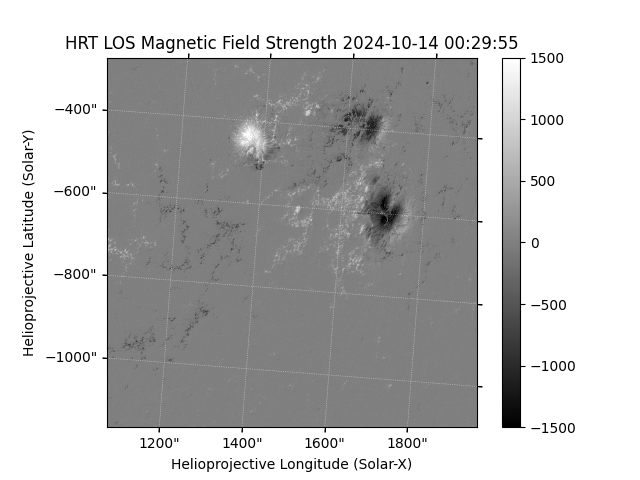
<matplotlib.colorbar.Colorbar object at 0x721a7cfdbd90>

Construct a Heliographic Stonyhurst header to reproject the image to. We use the Cylindrical Equal Area “CEA” projection (see section 5.2.2 of Calabretta and Greisen [2002]). For the Stonyhurst heliographic lines to be horizontal in this projection, the reference coordinate must be on the equator. We will be reprojecting using automatic extent determination, so the header needs only placeholder values for the shape.

hgs_center = SkyCoord(0, 0, unit=u.deg, frame="heliographic_stonyhurst",
                      obstime=blos_map.reference_date)
cea_scale = (0.03, 0.03) * u.deg / u.pix

cea_hdr = make_fitswcs_header(
    (0, 0),  # the shape values are only placeholders
    hgs_center,
    scale=cea_scale,
    projection_code="CEA",
    instrument=blos_map.instrument,
    wavelength=blos_map.wavelength,
)

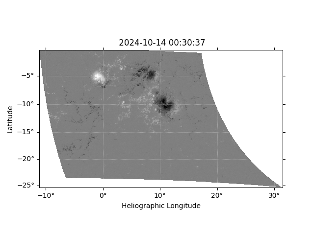
Reproject the map to the new header. By specifying auto_extent="edges", the extent of the reprojected map is automatically constructed by setting the appropriate array shape and reference pixel such that the reprojected extent contains the edges of the original map. Note that this treats the LOS magnetic field values as scalar image data. This is useful for visualisation, but it does not convert B_LOS into a radial or local heliographic magnetic field component.

outmap = blos_map.reproject_to(cea_hdr, algorithm="adaptive", kernel="Hann",
                               auto_extent="edges")

fig = plt.figure()
outmap.plot(norm=CenteredNorm(halfrange=1500, clip=True))

plt.show()

🏷 Tags: Map, Reproject, Solar Orbiter, SOAR, PHI