AIA to STEREO coordinate conversion

How to convert a point of a source on an AIA image to a position on a STEREO image.

import matplotlib.pyplot as plt

import astropy.units as u
from astropy.coordinates import SkyCoord

import sunpy.coordinates
import sunpy.map
from sunpy.data.sample import AIA_193_JUN2012, STEREO_A_195_JUN2012
from sunpy.sun import constants

Create a dictionary with the two maps, cropped down to full disk.

maps = {m.detector: m.submap(SkyCoord([-1100, 1100]*u.arcsec,
                                      [-1100, 1100]*u.arcsec,
                                      frame=m.coordinate_frame))
        for m in sunpy.map.Map([AIA_193_JUN2012, STEREO_A_195_JUN2012])}
maps['AIA'].plot_settings['vmin'] = 0  # set the minimum plotted pixel value

INFO: Missing metadata for solar radius: assuming the standard radius of the photosphere. [sunpy.map.mapbase]
INFO: Missing metadata for solar radius: assuming the standard radius of the photosphere. [sunpy.map.mapbase]

We will be transforming coordinates where the formation height of 304 A emission makes a difference, so we set the reference solar radius to 4 Mm above the solar surface (see Alissandrakis 2019).

for m in maps.values():
    m.meta['rsun_ref'] = (constants.radius + 4*u.Mm).to_value('m')

Plot both maps.

fig = plt.figure(figsize=(10, 4))
for i, m in enumerate(maps.values()):
    ax = fig.add_subplot(1, 2, i+1, projection=m)
    m.plot(axes=ax)

We are now going to pick out a region around the south west corner:

aia_bottom_left = SkyCoord(700 * u.arcsec,
                           100 * u.arcsec,
                           frame=maps['AIA'].coordinate_frame)
aia_top_right = SkyCoord(850 * u.arcsec,
                         350 * u.arcsec,
                         frame=maps['AIA'].coordinate_frame)

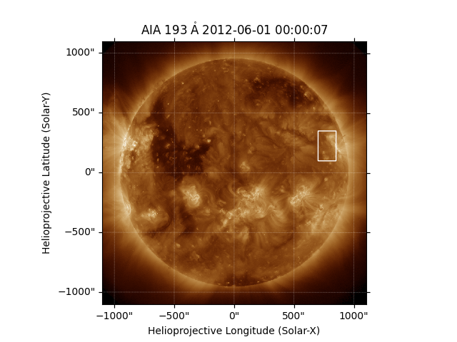
Plot a rectangle around the region we want to crop.

fig = plt.figure()
ax = fig.add_subplot(projection=maps['AIA'])
maps['AIA'].plot(axes=ax)
maps['AIA'].draw_quadrangle(aia_bottom_left, top_right=aia_top_right)

<astropy.visualization.wcsaxes.patches.Quadrangle object at 0x7f52d7838fa0>

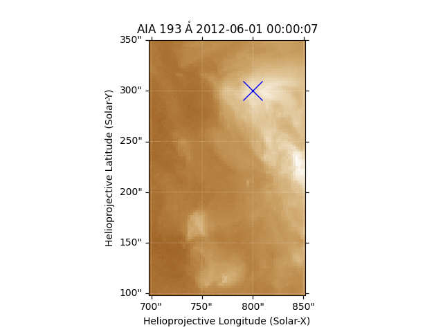
Create a submap of this area and draw an X at a specific feature of interest.

subaia = maps['AIA'].submap(aia_bottom_left, top_right=aia_top_right)
fig = plt.figure()
ax = fig.add_subplot(projection=subaia)
subaia.plot(axes=ax)

feature_aia = SkyCoord(800 * u.arcsec,
                       300 * u.arcsec,
                       frame=maps['AIA'].coordinate_frame)
ax.plot_coord(feature_aia, 'bx', fillstyle='none', markersize=20)

[<matplotlib.lines.Line2D object at 0x7f52d79b9360>]

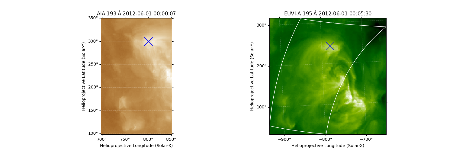
We can transform the coordinate of the feature to see its representation as seen by STEREO EUVI. The original coordinate did not contain a distance from the observer, so it is converted to a 3D coordinate assuming that it has a radius from Sun center equal to the reference solar radius of the coordinate frame, which we set earlier to be the formation height of 304 A emission.

print(feature_aia.transform_to(maps['EUVI'].coordinate_frame))

<SkyCoord (Helioprojective: obstime=2012-06-01T00:05:30.831, rsun=699700.0 km, observer=<HeliographicStonyhurst Coordinate (obstime=2012-06-01T00:05:30.831, rsun=699700.0 km): (lon, lat, radius) in (deg, deg, m)
    (116.29405786, 6.81772843, 1.43457186e+11)>): (Tx, Ty, distance) in (arcsec, arcsec, m)
    (-779.65052512, 243.90553172, 1.43047687e+11)>

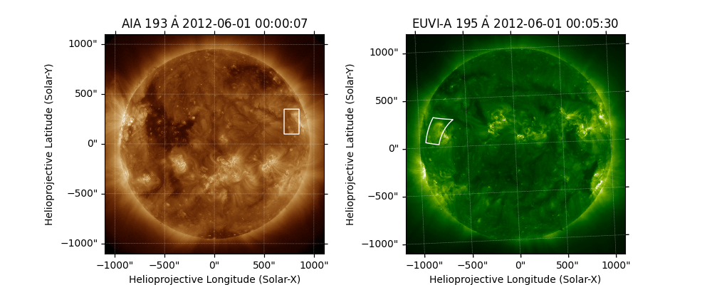
Now we can plot this box on both the AIA and EUVI images. Note that using draw_quadrangle() means that the plotted rectangle will be automatically warped appropriately to account for the different coordinate frames.

fig = plt.figure(figsize=(10, 4))

ax1 = fig.add_subplot(121, projection=maps['AIA'])
maps['AIA'].plot(axes=ax1)
maps['AIA'].draw_quadrangle(aia_bottom_left, top_right=aia_top_right, axes=ax1)

ax2 = fig.add_subplot(122, projection=maps['EUVI'])
maps['EUVI'].plot(axes=ax2)
maps['AIA'].draw_quadrangle(aia_bottom_left, top_right=aia_top_right, axes=ax2)

<astropy.visualization.wcsaxes.patches.Quadrangle object at 0x7f52d7742140>

We can now zoom in on the region in the EUVI image, and we also draw an X at the feature marked earlier. We do not need to explicitly transform the feature coordinate to the matching coordinate frame; that is performed automatically by plot_coord().

fig = plt.figure(figsize=(15, 5))

ax1 = fig.add_subplot(121, projection=subaia)
subaia.plot(axes=ax1)
ax1.plot_coord(feature_aia, 'bx', fillstyle='none', markersize=20)

subeuvi = maps['EUVI'].submap(aia_bottom_left, top_right=aia_top_right)

ax2 = fig.add_subplot(122, projection=subeuvi)
subeuvi.plot(axes=ax2)
maps['AIA'].draw_quadrangle(aia_bottom_left, top_right=aia_top_right, axes=ax2)
ax2.plot_coord(feature_aia, 'bx', fillstyle='none', markersize=20)

plt.show()