Note
Go to the end to download the full example code.
Artemis II Solar Eclipse#
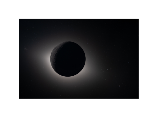
This example demonstrates how to process a solar eclipse image taken by the Artemis II crew.
This photo was taken using a digital camera onboard the spacecraft during their Lunar flyby on April 7, 2026. Due to the relative positions of the Artemis II spacecraft and the Moon, this eclipse provided nearly 54 minutes of totality, far exceeding what is possible on Earth.
This example walks through turning the photo, a plain JPEG with EXIF metadata
and no pointing information, into a Map with a Helioprojective WCS.
The observation time is constructed from the EXIF metadata, and the positions of
the Moon, Sun, and planets are retrieved from JPL Horizons.
The camera roll angle is refined by comparing the predicted and detected pixel
positions of Saturn, Mars, and Mercury, identified automatically.
Finally, the residual radial barrel distortion is modelled using a single
Simple Imaging Polynomial (SIP)
3rd order coefficient derived from the planet positions. With the resulting
calibrated Map it is straightforward to overplot some space-based
coronagraph data on top of the eclipse image.
Image credit: NASA/Artemis II crew
from pathlib import Path

import exifread
import hvpy
import matplotlib
import numpy as np
import requests
from hvpy.datasource import DataSource
from matplotlib import pyplot as plt
from matplotlib.patches import Circle
from scipy.signal import medfilt2d
from skimage import transform
from skimage.color import rgb2gray
from skimage.feature import canny, peak_local_max
from skimage.transform import hough_circle, hough_circle_peaks

import astropy.units as u
from astropy.coordinates import CartesianRepresentation, SkyCoord, solar_system_ephemeris
from astropy.time import Time
from astropy.visualization import simple_norm
from astropy.wcs import WCS

import sunpy.map
from sunpy.coordinates import Helioprojective, SphericalScreen, get_horizons_coord
from sunpy.map import Map
from sunpy.map.header_helper import make_fitswcs_header
from sunpy.util.config import get_and_create_download_dir

# Accurate planetary ephemeris from JPL Horizons
solar_system_ephemeris.set('de440s')
<ScienceState solar_system_ephemeris: 'de440s'>
Get and Convert the Raw Image#
The starting point is a single JPEG hosted in the NASA image library. It has no WCS, no pointing solution, or plate scale, we only have the raw image data.
We first download and read in the raw image data directly taken by the crew on Artemis-II and convert the RGB jpeg data to a grayscale image.
url = "https://images-assets.nasa.gov/image/art002e009301/art002e009301~orig.jpg"
filename = url.split("/")[-1]
with requests.get(url, stream=True) as res:
    res.raise_for_status()
    with open(filename, "wb") as f:
        for chunk in res.iter_content(chunk_size=8192):
            f.write(chunk)

artemis_image_rbg = np.flipud(matplotlib.image.imread(filename))
artemis_image = rgb2gray(artemis_image_rbg)
Let’s downsample the image to reasonable size for processing and
visualization. The original frame is very large, so for this example we
downsample by a factor of 6. This can be set to False if running locally
for full resolution analysis.
downsampled = True
if downsampled:
    artemis_image = transform.rescale(artemis_image, 1/6, anti_aliasing=True)
And now let’s plot the raw image.
fig, ax = plt.subplots()
ax.imshow(artemis_image_rbg, origin="lower")
ax.set_axis_off()
# Reduce memory usage on RTD build
del artemis_image_rbg
Extract Metadata#
Let’s now extract metadata stored in the JPEG image, in particular the date and time the image was taken. From another example (Artemis II trajectory), we know that Artemis II was in eclipse between 00:34 UTC and 01:29 UTC. Since the EXIF timestamp already falls within this range, we infer that it is already in UTC and should not have the EXIF time-zone offset applied.
with Path(filename).open("rb") as f:
    tags = exifread.process_file(f)

obsdate, obstime= tags['EXIF DateTimeDigitized'].values.split(" ")
obsdate = obsdate.replace(":", "-")
obstime = Time(f"{obsdate}T{obstime}")
print(obstime)

hours, _ = [int(part) for part in tags['EXIF OffsetTime'].values.split(":")]
offset = hours*u.hour

# obstime = obstime + offset  # Shift the time to UTC as needed
2026-04-07T01:06:19.000
Get Coordinates#
To get the coordinates of the Artemis II spacecraft, the Sun, the Moon, and
the planets at the observation time, we query JPL Horizons using
get_horizons_coord(). Here we use the NAIF IDs for
the bodies for the query, particularly because some of planet names do not
return a single match when supplied as strings.
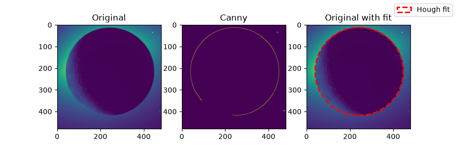
Find and Fit Moon’s Limb and Center#
While we now know where the Moon is on the sky, we still need to know where it is in the image. Fitting the Moon’s limb gives us that pixel location, and combined with the Moon’s known angular size, we can estimate the plate scale.
Here we use canny edge detection and circular Hough filtering to obtain the Moon’s limb and center. See the scikit-image documentation Circular and Elliptical Hough Transforms for more information on the functions used here.
First pass on a downscaled version is used to get an estimate, which is used to extract the region of interest (ROI) for full resolution pass.
print("starting low res pass")
scale = 0.5 if downsampled else 0.1
down_scaled = transform.rescale(artemis_image, scale, anti_aliasing=True)

 # Edge detection
edges = canny(down_scaled, sigma=2)

 # Radius range in scaled image (diameter ~1/3 of image height)
h, w = down_scaled.shape
radii = np.arange(0.25*h, 0.4*h, 10)

 # Hough
hough_res = hough_circle(edges, radii)
accums, cx, cy, rad = hough_circle_peaks(hough_res, radii, total_num_peaks=1)
del hough_res

 # Scale back to original resolution
moon_x = int(cx[0] / scale)
moon_y = int(cy[0] / scale)
moon_r = rad[0] / scale
roi_ext = int(1.05*moon_r)

slice_y = slice(moon_y-roi_ext, moon_y+roi_ext)
slice_x = slice(moon_x-roi_ext, moon_x+roi_ext)
print(f"Low res pass moon_x: {moon_x}, moon_y: {moon_y}, moon_r: {moon_r}")
starting low res pass
Low res pass moon_x: 556, moon_y: 478, moon_r: 229.0
Full resolution pass within ROI#
Let’s now re-run the limb fitting on the full resolution within the cropped ROI.
roi = artemis_image[slice_y, slice_x]

edges = canny(roi, sigma=2)

hough_radii = np.linspace(edges.shape[0] / 2.5, edges.shape[0] / 2, 30)
hough_res = hough_circle(edges, hough_radii).astype(np.float32) #  reduce peak memory usage

accums, cx, cy, radii = hough_circle_peaks(hough_res, hough_radii, total_num_peaks=1)

print(f"High res pass moon_x: {cx[0] + slice_x.start}, moon_y: {cy[0]+slice_y.start}, moon_r: {radii[0]}")
High res pass moon_x: 559, moon_y: 453, moon_r: 203.58620689655172
Plot edge detection and Hough filtering results#
fig, ax = plt.subplots(ncols=3, nrows=1, figsize=(9, 3))
ax[0].imshow(artemis_image[slice_y, slice_x])
ax[0].set_title("Original")
ax[1].imshow(edges)
ax[1].set_title("Canny")
circ = Circle(
    np.hstack([cx, cy]), radius=radii[0], facecolor="none", edgecolor="red",
    linewidth=2, linestyle="dashed", label="Hough fit")
ax[2].imshow(artemis_image[slice_y, slice_x])
ax[2].add_patch(circ)
ax[2].set_title("Original with fit")
fig.legend()
<matplotlib.legend.Legend object at 0x744f8c4887d0>
Create metadata#
Build up the metadata required to make a Map
Here we calculate the reference pixel, and plate scale.
im_cx = (cx[0] + slice_x.start) * u.pix
im_cy = (cy[0] + slice_y.start) * u.pix
im_radius = radii[0] * u.pix

moon = SkyCoord(coords['moon'], observer=coords['artemis_ii'])
R_moon = 0.2725076 *  u.R_earth  # IAU mean radius
dist_moon = SkyCoord(coords['artemis_ii']).separation_3d(moon)
moon_obs = np.arcsin(R_moon / dist_moon).to("arcsec")
print(moon_obs)

plate_scale = moon_obs / im_radius
print(plate_scale)
30309.259587263197 arcsec
148.87678320302047 arcsec / pix
Make a Map#
Make a Map using the metadata obtained so far using
make_fitswcs_header().
frame = Helioprojective(observer=coords['artemis_ii'], obstime=obstime)
moon_hpc = coords['moon'].transform_to(frame)

header = make_fitswcs_header(
    artemis_image,
    moon_hpc,
    reference_pixel=u.Quantity([im_cx, im_cy]),
    scale=u.Quantity([plate_scale, plate_scale])
)

artemis_map = Map(artemis_image, header)
Reusable plot helper
def plot_artemis_map(amap, moon_coord, planets, reset_lim=True, legend=True, figsize=(9,4), **kwargs):
    fig, ax = plt.subplots(1, 1, subplot_kw={"projection": amap}, figsize=figsize, **kwargs)
    amap.plot(axes=ax, norm=simple_norm(amap.data, 'power', min_percent=10, max_percent=99.9))
    amap.draw_limb(axes=ax, label='Sun')
    ax.coords[0].set_format_unit(u.deg)
    ax.coords[1].set_format_unit(u.deg)

    ax.plot_coord(moon_coord, 'b+', label="Lunar Center")
    theta = np.linspace(0, 360, 100) * u.deg
    lunar_limb = np.vstack([moon_hpc.Tx + np.sin(theta) * moon_obs, moon_hpc.Ty + np.cos(theta) * moon_obs])
    with SphericalScreen(amap.observer_coordinate):
        ax.plot_coord(SkyCoord(*lunar_limb, frame=amap.coordinate_frame), label="Lunar Limb")

    xlim = ax.get_xlim()
    ylim = ax.get_ylim()
    for name, coord in planets.items():
        ax.plot_coord(coord, 'o', markerfacecolor='none', label=name.title())
    if reset_lim:
        ax.set_xlim(xlim)
        ax.set_ylim(ylim)
    if legend:
        ax.legend(bbox_to_anchor=(1.05, 1), loc='upper left', borderaxespad=0)
    return fig, ax
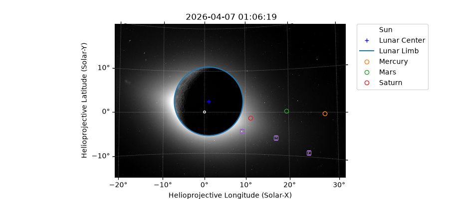
Plot map and positions of planets to see what should be visible
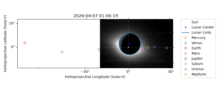
Mercury, Mars, Saturn and Neptune are within the field of view, though Neptune is not visible as it is too distant and faint.
Find roll angle#
A clear roll is visible, so the positions of the planets are used to
estimate the camera orientation. Use skimage.feature.peak_local_max()
to find the brightest peaks, which should correspond to the planets.
if downsampled:
    planets_pixels = peak_local_max(artemis_image, threshold_abs=0.9, num_peaks=3, min_distance=30)
else:
    artemis_median_img = medfilt2d(artemis_image, kernel_size=5)
    planets_pixels = peak_local_max(artemis_median_img, threshold_abs=0.9, num_peaks=3, min_distance=30)
    del artemis_median_img

planets_pix_x = planets_pixels[:,1]
planets_pix_y = planets_pixels[:,0]

planet_coords = artemis_map.pixel_to_world(planets_pix_x * u.pix, planets_pix_y * u.pix)
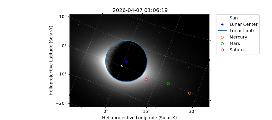
Verify we’ve correctly identified the planets.
fig, ax = plot_artemis_map(artemis_map, moon_hpc, planets)
with SphericalScreen(coords["artemis_ii"]):
    ax.plot_coord(planet_coords, 's', markerfacecolor='none')
We need to determine which pixel positions correspond to which planets. From the map above, we can see that, in terms of distance from the Moon, the planets are Saturn, Mars, and Mercury, in that order. Therefore, we sort them by the separation angle from the Moon’s center.
# Saturn, Mars, Mercury
with SphericalScreen(coords["artemis_ii"]):
    sep = moon_hpc.transform_to(planet_coords.frame).separation(planet_coords)
planet_index = np.argsort(sep)
actual_planets_pixel = CartesianRepresentation(planets_pix_x[planet_index], planets_pix_y[planet_index], [0] * 3) * u.pix

moon_pixel = CartesianRepresentation(*artemis_map.wcs.world_to_pixel(moon_hpc), 0)*u.pix

# to match the order of the actual_planets_pixel
planets_temp = SkyCoord([planets[name] for name in ["saturn", "mars", "mercury"]])
planets_pixel = CartesianRepresentation(*artemis_map.wcs.world_to_pixel(planets_temp), 0) * u.pix

vec_expected = planets_pixel - moon_pixel
vec_actual = actual_planets_pixel - moon_pixel
roll_angles = -np.arccos(vec_expected.dot(vec_actual) / (vec_expected.norm() * vec_actual.norm()))
print(roll_angles.to('deg'))

weights = sep[planet_index].to(u.deg).value
roll_angles_weighted = np.average(roll_angles, weights=weights).to('deg')
print(f"Weighted roll: {roll_angles_weighted:.4f}")
[-20.60914096 -21.16794785 -21.33334763] deg
Weighted roll: -21.1349 deg
Use derived roll and make new header and map
header_roll = make_fitswcs_header(
    artemis_image,
    moon_hpc,
    reference_pixel=u.Quantity([im_cx, im_cy]),
    scale=u.Quantity([plate_scale, plate_scale]),
    rotation_angle=-roll_angles_weighted
)

artemis_map_roll = Map(artemis_image, header_roll)
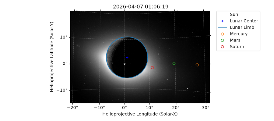
Let’s now plot map and positions of Saturn, Mars, and Mercury to check if the WCS is correct.
There seems to be some residual distortion that gets worse towards the edges.
Correct Optical Distortion#
We can see that there is some optical distortion. Let’s assume the distortion is due to the lens (e.g., barrel or pincushion), centered in the middle of the image, and derive the correction from the observed versus actual planet positions.
cx, cy = artemis_map_roll.wcs.wcs.crpix
r_actual, r_predicted = [], []
for i, name in enumerate(["saturn", "mars", "mercury"]):
    hpc = planets[name].transform_to(artemis_map_roll.coordinate_frame)
    px, py = artemis_map_roll.wcs.world_to_pixel(hpc)
    ax, ay = planets_pix_x[planet_index][i], planets_pix_y[planet_index][i]
    r_predicted.append(np.sqrt((px - cx)**2 + (py - cy)**2))
    r_actual.append(np.sqrt((ax - cx)**2 + (ay - cy)**2))

r_predicted = np.array(r_predicted)
r_actual    = np.array(r_actual)

k1_estimates = (r_actual/r_predicted - 1) / r_predicted**2
weights = r_predicted  # weight by distance — Mercury most reliable
k1 = np.average(k1_estimates, weights=weights)
print(f"k1 per planet: {k1_estimates}")
print(f"Weighted k1:   {k1:.6e} pix^-2")

# Use only Mars and Mercury — Saturn too close to center and fit error
k1_estimates_reliable = k1_estimates[1:]
r_reliable = r_predicted[1:]
k1 = np.average(k1_estimates_reliable, weights=r_reliable)
print(f"k1 (Mars+Mercury only): {k1:.6e} pix^-2")
k1 per planet: [-8.04017444e-09 -8.93987754e-08 -7.14795984e-08]
Weighted k1:   -6.545246e-08 pix^-2
k1 (Mars+Mercury only): -7.866379e-08 pix^-2
Create a SIP header, WCS and verify the SIP improve positions
header_sip = artemis_map_roll.fits_header.copy()
header_sip['CTYPE1'] = 'HPLN-TAN-SIP'
header_sip['CTYPE2'] = 'HPLT-TAN-SIP'
header_sip['A_ORDER'] = 3
header_sip['B_ORDER'] = 3
header_sip['A_3_0'] = -k1
header_sip['A_1_2'] = -k1
header_sip['B_0_3'] = -k1
header_sip['B_2_1'] = -k1
header_sip['A_DMAX'] = 1.0
header_sip['B_DMAX'] = 1.0
wcs_sip = WCS(header_sip)

for i, name in enumerate(["saturn", "mars", "mercury"]):
     hpc = planets[name].transform_to(artemis_map_roll.coordinate_frame)
     px_nosip = wcs_sip.wcs_world2pix([[hpc.Tx.to(u.deg).value, hpc.Ty.to(u.deg).value]], 0)[0]
     px_sip   = wcs_sip.all_world2pix([[hpc.Tx.to(u.deg).value, hpc.Ty.to(u.deg).value]], 0)[0]
     ax, ay   = planets_pix_x[planet_index][i], planets_pix_y[planet_index][i]
     print(f"{name}: residual without SIP=({ax-px_nosip[0]:.1f}, {ay-px_nosip[1]:.1f})  "
           f"with SIP=({ax-px_sip[0]:.1f}, {ay-px_sip[1]:.1f})")
saturn: residual without SIP=(1.6, 1.9)  with SIP=(2.6, 0.9)
mars: residual without SIP=(-8.1, 4.1)  with SIP=(-1.4, 0.5)
mercury: residual without SIP=(-22.6, 9.0)  with SIP=(-1.2, -2.0)
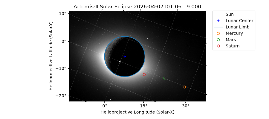
Final Map#
Create a final version of the map with the SIP headers.
artemis_map_final = Map((artemis_image, header_sip))
fig, ax = plot_artemis_map(artemis_map_final, moon_hpc, planets)
ax.set_title(f"Artemis-II Solar Eclipse {obstime}")
fig.tight_layout()
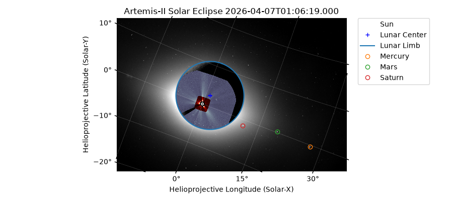
Overplotting Coronagraph Images#
In this section we will fetch images of the near corona from SOHO/LASCO and overplot them on the eclipse map. The Artemis II image shows the faint outer corona around the Moon, as the spacecraft was close to the moon during the flyby, so the apparent angular size is much larger than the Sun’s, so it blocks not only the Sun’s disk but a substantial region of the inner corona around it.
By reprojecting and overplotting the LASCO images, we can overlap them inside the Moon’s image, to produce a composite that extends from the inner corona outwards.
First step is to fetch the images from Helioviewer.
lasco_c2_file = hvpy.save_file(hvpy.getJP2Image(obstime.datetime,
                                                DataSource.LASCO_C2.value),
                               filename=get_and_create_download_dir() + "/LASCO_C2.jp2", overwrite=True)
lasco_c2_map = Map(lasco_c2_file)
lasco_c3_file = hvpy.save_file(hvpy.getJP2Image(obstime.datetime,
                                                DataSource.LASCO_C3.value),
                               filename=get_and_create_download_dir() + "/LASCO_C3.jp2", overwrite=True)
lasco_c3_map = Map(lasco_c3_file)
Next we reproject the LASCO map to the same WCS as the Artemis eclipse map.
with SphericalScreen(coords["artemis_ii"]):
    c3_map_img = lasco_c3_map.reproject_to(artemis_map_final.wcs)
    c2_map_img = lasco_c2_map.reproject_to(artemis_map_final.wcs)
/home/docs/checkouts/readthedocs.org/user_builds/sunpy/conda/latest/lib/python3.13/site-packages/sunpy/map/mapbase.py:671: SunpyMetadataWarning: Missing metadata for observer: assuming Earth-based observer.
For frame 'heliographic_stonyhurst' the following metadata is missing: hglt_obs,dsun_obs,hgln_obs
For frame 'heliographic_carrington' the following metadata is missing: crln_obs,crlt_obs,dsun_obs

  obs_coord = self.observer_coordinate
As the final step we will crop the LASCO C3 image to the limb of the Moon and mask regions with no data.
# Calculate coordinates for each pixel in the map.
all_hpc = sunpy.map.all_coordinates_from_map(c3_map_img)

# Calculate the angular offset from the center of the moon for each pixel.
moon_cen_offsets = all_hpc.separation(coords['moon'], origin_mismatch='ignore')

# Create a mask which is True for all offsets greater than the
# observed angular width of the moon.
c3_map_img.mask = np.logical_or(
    moon_cen_offsets >= moon_obs,
    # Also mask out the parts of the image with no data
    c3_map_img.data < 10,
)
# Mask out the parts of the C2 image with no data
c2_map_img.mask = c2_map_img.data < 10
Now setup a new plot with the same distortion corrected eclipse image and reprojected, masked LASCO data.
fig, ax = plot_artemis_map(artemis_map_final, moon_hpc, planets)

# Overplot both LASCO images
c3_map_img.plot(axes=ax)
c2_map_img.plot(axes=ax)

ax.set_title(f"Artemis-II Solar Eclipse {obstime}")
fig.tight_layout()
Total running time of the script: (0 minutes 17.490 seconds)