Maps#
In this section of the tutorial, you will learn about the Map object.
Map objects hold two-dimensional data along with the accompanying metadata.
They can be used with any two-dimensional data array with two spatial axes and FITS-compliant metadata.
As you will see in this tutorial, the primary advantage of using a Map object over a bare NumPy array is the ability to perform coordinate aware operations on the underlying array, such as rotating the Map to remove the roll angle of an instrument or cropping a Map to a specific field of view.
Additionally, because Map is capable of ingesting data from many different sources, it provides a common interface for any two-dimensional data product.
By the end of this tutorial, you will learn how to create a Map, access the underlying data and metadata, convert between physical coordinates and pixel coordinates of a Map, and the basics of visualizing a Map.
Additionally, you will learn how to combine multiple Maps into a MapSequence or a CompositeMap.
Note
In this section and in Timeseries, we will use the sample data included with sunpy.
These data are primarily useful for demonstration purposes or simple debugging.
These files have names like sunpy.data.sample.AIA_171_IMAGE and sunpy.data.sample.RHESSI_IMAGE and are automatically downloaded to your computer as you need them.
Once downloaded, these sample data files will be paths to their location on your computer.
Creating Maps#
To create a Map from a sample Atmospheric Imaging Assembly (AIA) image,
>>> import sunpy.map
>>> import sunpy.data.sample

>>> sunpy.data.sample.AIA_171_IMAGE
PosixPath('.../AIA20110607_063302_0171_lowres.fits')
>>> my_map = sunpy.map.Map(sunpy.data.sample.AIA_171_IMAGE)
In many cases sunpy automatically detects the type of file as well as the the instrument associated with it.
In this case, we have a FITS file from the AIA instrument onboard the Solar Dynamics Observatory (SDO).
To make sure this has all worked correctly, we can take a quick look at my_map,
>>> my_map
<sunpy.map.sources.sdo.AIAMap object at ...>
SunPy Map
---------
Observatory:                 SDO
Instrument:          AIA 3
Detector:            AIA
Measurement:                 171.0 Angstrom
Wavelength:          171.0 Angstrom
Observation Date:    2011-06-07 06:33:02
Exposure Time:               0.234256 s
Dimension:           [1024. 1024.] pix
Coordinate System:   helioprojective
Scale:                       [2.402792 2.402792] arcsec / pix
Reference Pixel:     [511.5 511.5] pix
Reference Coord:     [3.22309951 1.38578135] arcsec
array([[ -95.92475  ,    7.076416 ,   -1.9656711, ..., -127.96519  ,
        -127.96519  , -127.96519  ],
       [ -96.97533  ,   -5.1167884,    0.       , ...,  -98.924576 ,
        -104.04137  , -127.919716 ],
       [ -93.99607  ,    1.0189276,   -4.0757103, ...,   -5.094638 ,
         -37.95505  , -127.87541  ],
       ...,
       [-128.01454  , -128.01454  , -128.01454  , ..., -128.01454  ,
        -128.01454  , -128.01454  ],
       [-127.899666 , -127.899666 , -127.899666 , ..., -127.899666 ,
        -127.899666 , -127.899666 ],
       [-128.03072  , -128.03072  , -128.03072  , ..., -128.03072  ,
        -128.03072  , -128.03072  ]], shape=(1024, 1024), dtype=float32)
This should show a representation of the data as well as some of its associated attributes.
If you are in a Jupyter Notebook, this will show a rich HTML view of the table along with several quick-look plots.
Otherwise, you can use the quicklook() method to see these quick-look plots.
>>> my_map.quicklook()
<sunpy.map.sources.sdo.AIAMap object at 0x744f5dbc5550>
|
Image colormap uses histogram equalization
Click on the image to toggle between units 
|
||||||||||||||||||||||||

|
Inspecting Map Metadata#
The metadata for a Map is exposed via attributes on the Map.
These attributes can be accessed by typing my_map.<attribute-name>.
For example, to access the date of the observation,
>>> my_map.date
<Time object: scale='utc' format='isot' value=2011-06-07T06:33:02.770>
Notice that this is an Time object which we discussed in the previous Times section of the tutorial.
Similarly, we can access the exposure time of the image,
>>> my_map.exposure_time
<Quantity 0.234256 s>
Notice that this returns an Quantity object which we discussed in the previous Units section of the tutorial.
The full list of attributes can be found in the reference documentation for GenericMap.
These metadata attributes are all derived from the underlying FITS metadata, but are represented as rich Python objects, rather than simple strings or numbers.
Map Data#
The data in a Map is stored as a numpy.ndarray object and is accessible through the data attribute:
>>> my_map.data
array([[ -95.92475  ,    7.076416 ,   -1.9656711, ..., -127.96519  ,
    -127.96519  , -127.96519  ],
   [ -96.97533  ,   -5.1167884,    0.       , ...,  -98.924576 ,
    -104.04137  , -127.919716 ],
   [ -93.99607  ,    1.0189276,   -4.0757103, ...,   -5.094638 ,
     -37.95505  , -127.87541  ],
   ...,
   [-128.01454  , -128.01454  , -128.01454  , ..., -128.01454  ,
    -128.01454  , -128.01454  ],
   [-127.899666 , -127.899666 , -127.899666 , ..., -127.899666 ,
    -127.899666 , -127.899666 ],
   [-128.03072  , -128.03072  , -128.03072  , ..., -128.03072  ,
    -128.03072  , -128.03072  ]], shape=(1024, 1024), dtype=float32)
This array can then be indexed like any other NumPy array. For example, to get the 0th element in the array:
>>> my_map.data[0, 0]
np.float32(-95.92475)
The first index corresponds to the y direction and the second to the x direction in the two-dimensional pixel coordinate system. For more information about indexing, please refer to the numpy documentation.
Data attributes like dimensionality and type are also accessible as attributes on my_map:
>>> my_map.dimensions
PixelPair(x=<Quantity 1024. pix>, y=<Quantity 1024. pix>)
>>> my_map.dtype
dtype('float32')
Additionally, there are several methods that provide basic summary statistics of the data:
>>> my_map.min()
np.float32(-129.78036)
>>> my_map.max()
np.float32(192130.17)
>>> my_map.mean()
np.float32(427.02252)
Coordinates, and the World Coordinate System#
In Coordinates, you learned how to define coordinates with SkyCoord using different solar coordinate frames.
The coordinate frame of a Map is provided as an attribute,
>>> my_map.coordinate_frame
<Helioprojective Frame (obstime=2011-06-07T06:33:02.880, rsun=696000.0 km, observer=<HeliographicStonyhurst Coordinate (obstime=2011-06-07T06:33:02.880, rsun=696000.0 km): (lon, lat, radius) in (deg, deg, m)
    (-0.00406429, 0.04787238, 1.51846026e+11)>)>
This tells us that the coordinate system of the image is Helioprojective (HPC) and that it is defined by an observer at a particular location. This observer coordinate is also provided as an attribute,
>>> my_map.observer_coordinate
<SkyCoord (HeliographicStonyhurst: obstime=2011-06-07T06:33:02.880, rsun=696000.0 km): (lon, lat, radius) in (deg, deg, m)
    (-0.00406429, 0.04787238, 1.51846026e+11)>
This tells us the location of the spacecraft, in this case SDO, when it recorded this particular observation, as derived from the FITS metadata.
Map has several additional coordinate-related attributes that provide the coordinates of the center and corners of the Map,
>>> my_map.center
<SkyCoord (Helioprojective: obstime=2011-06-07T06:33:02.880, rsun=696000.0 km, observer=<HeliographicStonyhurst Coordinate (obstime=2011-06-07T06:33:02.880, rsun=696000.0 km): (lon, lat, radius) in (deg, deg, m)
    (-0.00406429, 0.04787238, 1.51846026e+11)>): (Tx, Ty) in arcsec
    (3.22309951, 1.38578135)>
>>> my_map.bottom_left_coord
<SkyCoord (Helioprojective: obstime=2011-06-07T06:33:02.880, rsun=696000.0 km, observer=<HeliographicStonyhurst Coordinate (obstime=2011-06-07T06:33:02.880, rsun=696000.0 km): (lon, lat, radius) in (deg, deg, m)
    (-0.00406429, 0.04787238, 1.51846026e+11)>): (Tx, Ty) in arcsec
    (-1228.76466158, -1224.62447509)>
>>> my_map.top_right_coord
<SkyCoord (Helioprojective: obstime=2011-06-07T06:33:02.880, rsun=696000.0 km, observer=<HeliographicStonyhurst Coordinate (obstime=2011-06-07T06:33:02.880, rsun=696000.0 km): (lon, lat, radius) in (deg, deg, m)
    (-0.00406429, 0.04787238, 1.51846026e+11)>): (Tx, Ty) in arcsec
    (1235.21095899, 1227.39598836)>
But what if we wanted to know what pixel these physical coordinates correspond to?
Each Map has an associated World Coordinate System, or WCS, which is derived from the underlying metadata and expressed as an astropy.wcs.WCS object.
The WCS is accessible as an attribute:
>>> my_map.wcs
WCS Keywords

Number of WCS axes: 2
CTYPE : 'HPLN-TAN' 'HPLT-TAN'
CUNIT : 'deg' 'deg'
CRVAL : 0.00089530541880571 0.00038493926472939
CRPIX : 512.5 512.5
PC1_1 PC1_2  : 0.99999706448085 0.0024230207763071
PC2_1 PC2_2  : -0.0024230207763071 0.99999706448085
CDELT : 0.00066744222222222 0.00066744222222222
NAXIS : 1024  1024
WCS is a fairly complex topic, but all we need to know for now is that the WCS provides the transformation between the pixel coordinates of the image and physical or “world” coordinates.
In particular, we will only focus on two methods: world_to_pixel and pixel_to_world.
First, let’s find the pixel location corresponding to the center of the Map,
>>> center_pixel = my_map.wcs.world_to_pixel(my_map.center)
>>> center_pixel
(array(511.5), array(511.5))
Notice that these coordinates are not necessarily integers. The corresponding pixel-to-world transformation should then give us back our center coordinate from above,
>>> my_map.wcs.pixel_to_world(center_pixel[0], center_pixel[1])
<SkyCoord (Helioprojective: obstime=2011-06-07T06:33:02.880, rsun=696000.0 km, observer=<HeliographicStonyhurst Coordinate (obstime=2011-06-07T06:33:02.880, rsun=696000.0 km): (lon, lat, radius) in (deg, deg, m)
    (-0.00406429, 0.04787238, 1.51846026e+11)>): (Tx, Ty) in arcsec
    (3.22309951, 1.38578135)>
As another example, if we transform the center of the lower-left pixel to a world coordinate, it should correspond to bottom left coordinate from above,
>>> my_map.wcs.pixel_to_world(0, 0)
<SkyCoord (Helioprojective: obstime=2011-06-07T06:33:02.880, rsun=696000.0 km, observer=<HeliographicStonyhurst Coordinate (obstime=2011-06-07T06:33:02.880, rsun=696000.0 km): (lon, lat, radius) in (deg, deg, m)
    (-0.00406429, 0.04787238, 1.51846026e+11)>): (Tx, Ty) in arcsec
    (-1228.76466158, -1224.62447509)>
These two methods are extremely useful when trying to understand which pixels correspond to which physical coordinates or when trying to locate the same physical location in images taken by separate spacecraft.
Visualizing Maps#
In the Creating Maps section, you learned how to generate a quicklook summary of a Map.
However, the Map object also has a plot() method that allows for more fine-grained control over how the Map is visualized and is especially useful for generating publication-quality plots.
In this section of the tutorial, you will learn how to build up an increasingly detailed visualization of a Map, including adjusting the colormap and normalization and and overlaying coordinates and contours.
Basic Plotting#
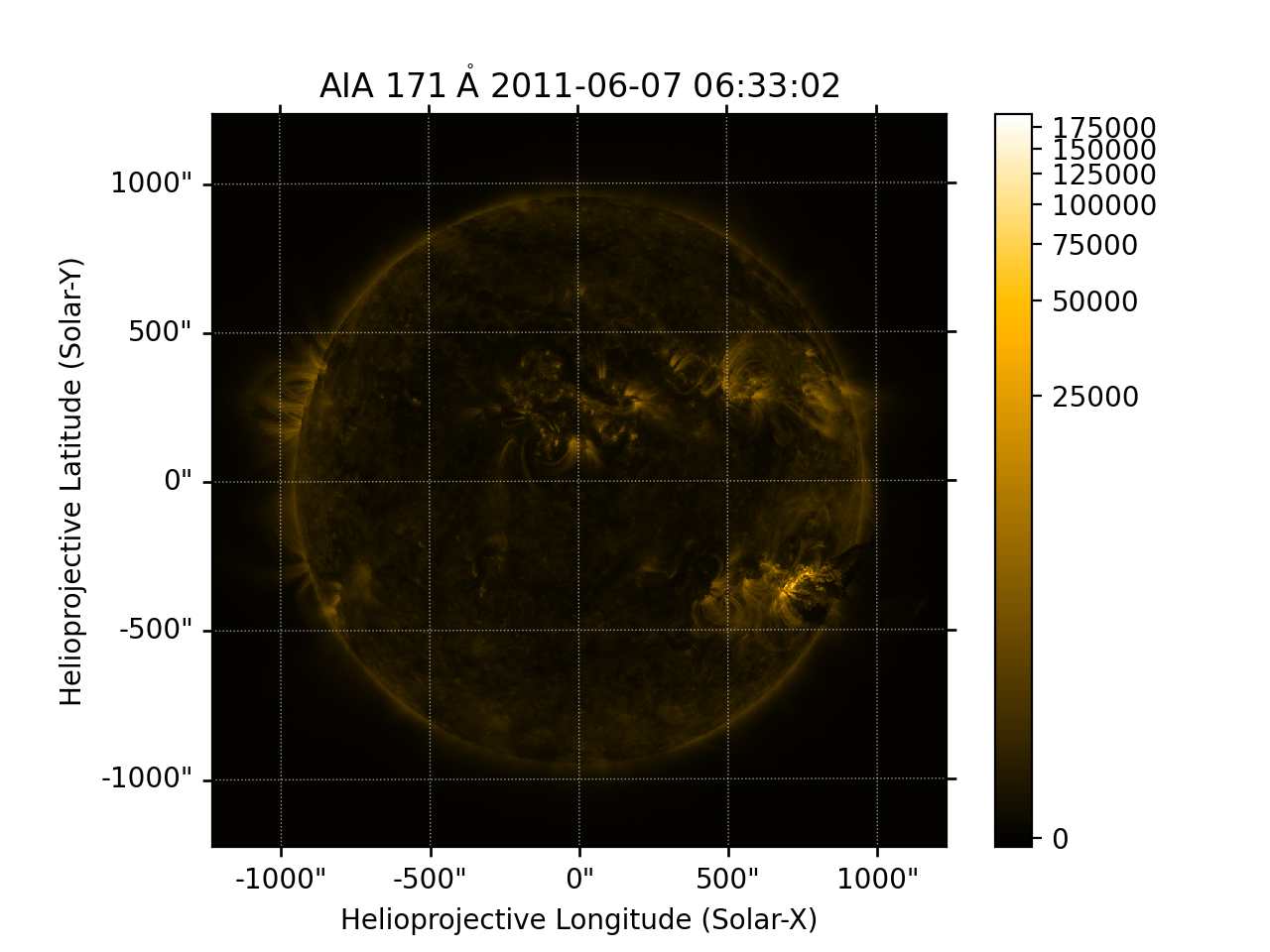
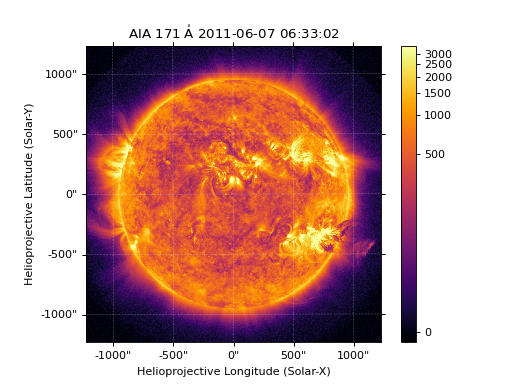
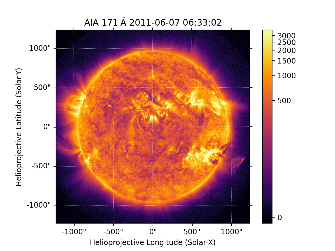
First, let’s create a basic plot of our Map, including a colorbar,
import matplotlib.pyplot as plt

fig = plt.figure()
ax = fig.add_subplot(projection=my_map)
my_map.plot(axes=ax)
plt.colorbar()
plt.show()
(Source code, png, hires.png, pdf)
Note
We imported matplotlib.pyplot in order to create the figure and the axis we plotted on our map onto.
Under the hood, sunpy uses matplotlib to visualize the image meaning that plots built with sunpy can be further customized using matplotlib.
However, for the purposes of this tutorial, you do not need to be familiar with Matplotlib.
For a series of detailed examples showing how to customize your Map plots, see the Plotting section of the Example Gallery as well as the documentation for astropy.visualization.wcsaxes.
Note that the title and colormap have been set by sunpy based on the observing instrument and wavelength. Furthermore, the tick and axes labels have been automatically set based on the coordinate system of the Map.
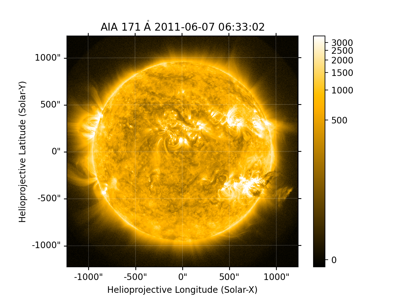
Looking at the plot above, you likely notice that the resulting image is a bit dim.
To fix this, we can use the clip_interval keyword to automatically adjust the colorbar limits to clip out the dimmest 1% and the brightest 0.5% of pixels.
fig = plt.figure()
ax = fig.add_subplot(projection=my_map)
my_map.plot(axes=ax, clip_interval=(1, 99.5)*u.percent)
plt.colorbar()
plt.show()
(Source code, png, hires.png, pdf)

Changing the Colormap and Normalization#
Historically, particular colormaps are assigned to images based on what instrument they are from and what wavelength is being observed. By default, sunpy will select the colormap based on the available metadata. This default colormap is available as an attribute,
>>> my_map.cmap.name
'sdoaia171'
When visualizing a Map, you can change the colormap using the cmap keyword argument.
For example, you can use the ‘inferno’ colormap from matplotlib:
fig = plt.figure()
ax = fig.add_subplot(projection=my_map)
my_map.plot(axes=ax, cmap='inferno', clip_interval=(1,99.5)*u.percent)
plt.colorbar()
plt.show()
(Source code, png, hires.png, pdf)

Note
sunpy provides specific colormaps for many different instruments.
For a list of all colormaps provided by sunpy, see the documentation for sunpy.visualization.colormaps.
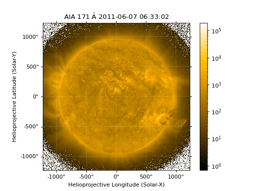
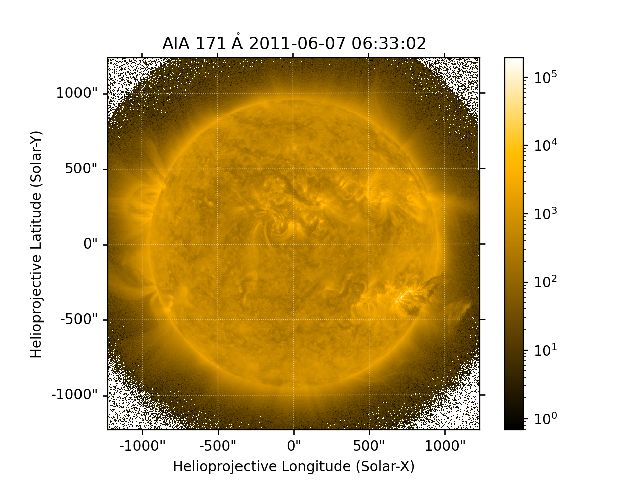
The normalization, or the mapping between the data values and the colors in our colormap, is also determined based on the underlying metadata.
Notice that in the plots we’ve made so far, the ticks on our colorbar are not linearly spaced.
Just like in the case of the colormap, we can use a normalization other than the default by passing a keyword argument to the plot() method.
For example, we can use a logarithmic normalization instead:
import matplotlib.colors

fig = plt.figure()
ax = fig.add_subplot(projection=my_map)
my_map.plot(norm=matplotlib.colors.LogNorm())
plt.colorbar()
plt.show()
(Source code, png, hires.png, pdf)

Note
You can also view or make changes to the default settings through the sunpy.map.GenericMap.plot_settings dictionary.
See Editing the colormap and normalization of a Map for an example of of how to change the default plot settings.
Overlaying Contours and Coordinates#
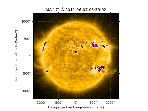
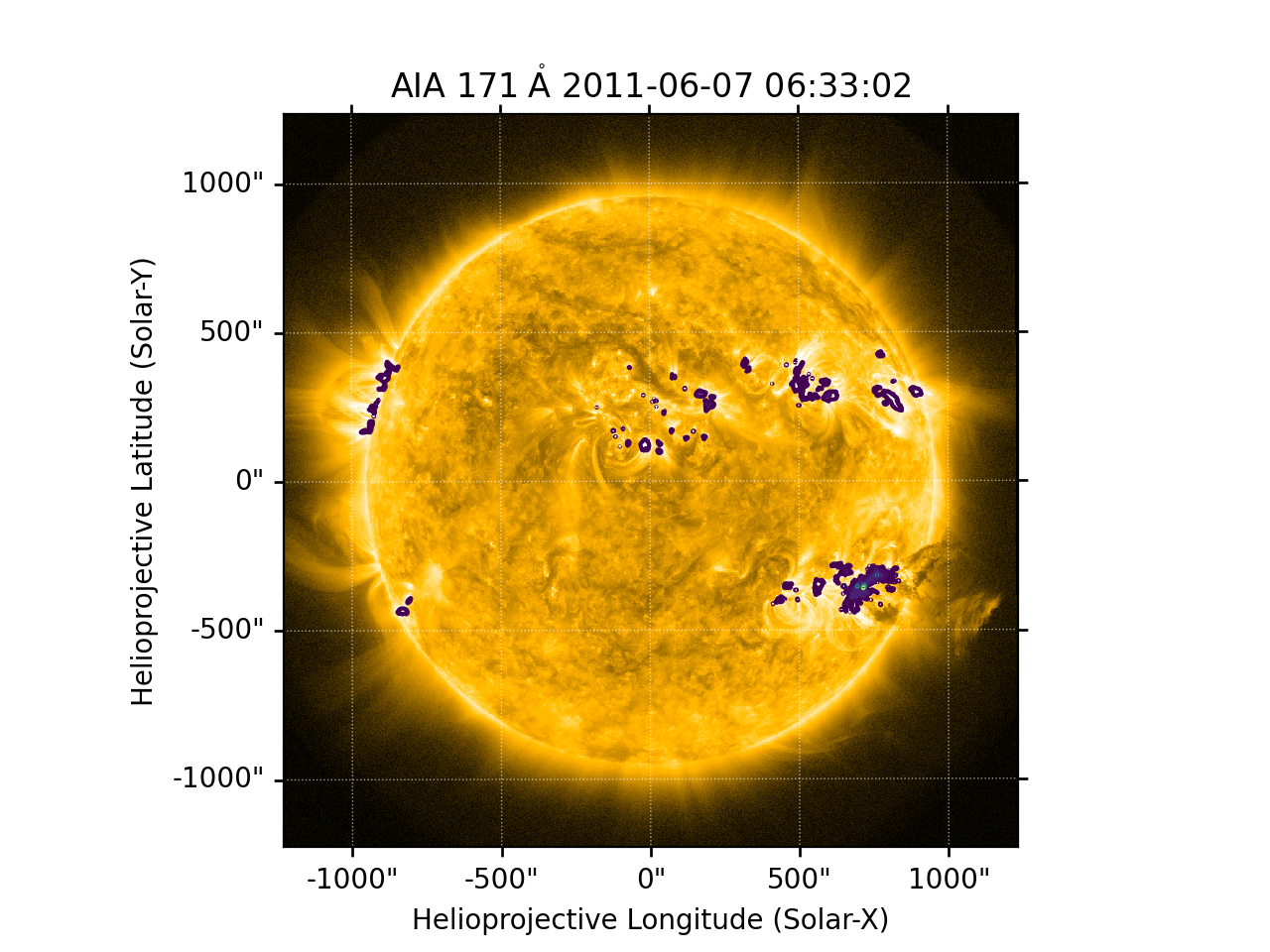
When plotting images, we often want to highlight certain features or overlay certain data points. There are several methods attached to Map that make this task easy. For example, we can draw contours around the brightest 0.5% percent of pixels in the image:
fig = plt.figure()
ax = fig.add_subplot(projection=my_map)
my_map.plot(axes=ax, clip_interval=(1,99.5)*u.percent)
my_map.draw_contours([2, 5, 10, 50, 90] * u.percent, axes=ax)
plt.show()
(Source code, png, hires.png, pdf)

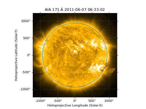
Additionally, the solar limb, as determined by the location of the observing instrument at the time of the observation, can be easily overlaid on an image:
fig = plt.figure()
ax = fig.add_subplot(projection=my_map)
my_map.plot(axes=ax, clip_interval=(1,99.5)*u.percent)
my_map.draw_limb(axes=ax, color='C0')
plt.show()
(Source code, png, hires.png, pdf)
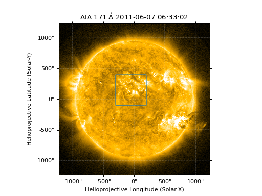
We can also overlay a box denoting a particular a region of interest as expressed in world coordinates using the the coordinate frame of our image:
roi_bottom_left = SkyCoord(Tx=-300*u.arcsec, Ty=-100*u.arcsec, frame=my_map.coordinate_frame)
roi_top_right = SkyCoord(Tx=200*u.arcsec, Ty=400*u.arcsec, frame=my_map.coordinate_frame)
fig = plt.figure()
ax = fig.add_subplot(projection=my_map)
my_map.plot(axes=ax, clip_interval=(1,99.5)*u.percent)
my_map.draw_quadrangle(roi_bottom_left, top_right=roi_top_right, axes=ax, color='C0')
plt.show()
(Source code, png, hires.png, pdf)

Because our visualization knows about the coordinate system of our Map, it can transform any coordinate to the coordinate frame of our Map and then use the underlying WCS that we discussed in the Coordinates, and the World Coordinate System section to translate this to a pixel position.
This makes it simple to plot any coordinate on top of our Map using the plot_coord() method.
The following example shows how to plot some points on our Map, including the center coordinate of our Map:
coords = SkyCoord(Tx=[100,1000] * u.arcsec, Ty=[100,1000] * u.arcsec, frame=my_map.coordinate_frame)

fig = plt.figure()
ax = fig.add_subplot(projection=my_map)
my_map.plot(axes=ax, clip_interval=(1,99.5)*u.percent)
ax.plot_coord(coords, 'o')
ax.plot_coord(my_map.center, 'X')
plt.show()
(Source code, png, hires.png, pdf)

Note
Map visualizations can be heavily customized using both matplotlib and astropy.visualization.wcsaxes.
See the Plotting section of the Example Gallery for more detailed examples of how to customize Map visualizations.
Cropping Maps and Combining Pixels#
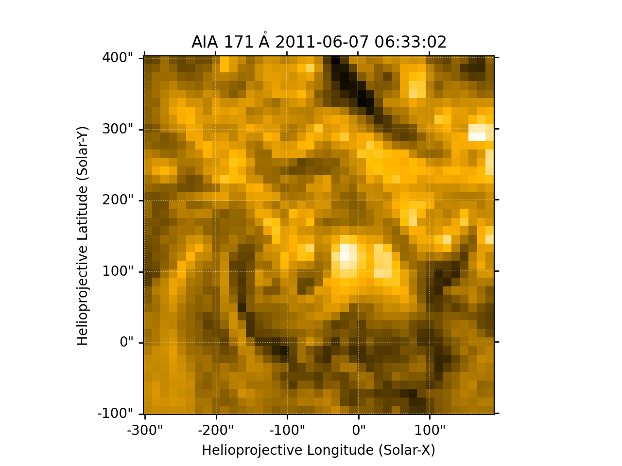
In analyzing images of the Sun, we often want to choose a smaller portion of the full disk to look at more closely. Let’s use the region of interest we defined above to crop out that portion of our image:
my_submap = my_map.submap(roi_bottom_left, top_right=roi_top_right)

fig = plt.figure()
ax = fig.add_subplot(projection=my_submap)
my_submap.plot(axes=ax)
plt.show()
(Source code, png, hires.png, pdf)

Additionally, we also may want to combine multiple pixels into a single pixel (a “superpixel”) to, for example, increase our signal-to-noise ratio.
We can accomplish this with the superpixel method by specifying how many pixels, in each dimension, we want our new superpixels to contain.
For example, we can combine 4 pixels in each dimension such that our new superpixels contain 16 original pixels:
my_super_submap = my_submap.superpixel((5,5)*u.pixel)

fig = plt.figure()
ax = fig.add_subplot(projection=my_super_submap)
my_super_submap.plot(axes=ax)
plt.show()
(Source code, png, hires.png, pdf)

Note
Map provides additional methods for manipulating the underlying image data.
See the reference documentation for GenericMap for a complete list of available methods as well as the Map section of the Example Gallery for more detailed examples.
Map Sequences#
While GenericMap can only contain a two-dimensional array and metadata corresponding to a single observation, a MapSequence is comprised of an ordered list of maps.
By default, the Maps are ordered by their observation date, from earliest to latest date.
A MapSequence can be created by supplying multiple existing maps:
>>> another_map = sunpy.map.Map(sunpy.data.sample.EIT_195_IMAGE)
>>> map_seq = sunpy.map.Map([my_map, another_map], sequence=True)
A map sequence can be indexed in the same manner as a list. For example, the following returns the same information as in Creating Maps:
>>> map_seq.maps[0]
<sunpy.map.sources.sdo.AIAMap object at ...>
SunPy Map
---------
Observatory:                 SDO
Instrument:          AIA 3
Detector:            AIA
Measurement:                 171.0 Angstrom
Wavelength:          171.0 Angstrom
Observation Date:    2011-06-07 06:33:02
Exposure Time:               0.234256 s
Dimension:           [1024. 1024.] pix
Coordinate System:   helioprojective
Scale:                       [2.402792 2.402792] arcsec / pix
Reference Pixel:     [511.5 511.5] pix
Reference Coord:     [3.22309951 1.38578135] arcsec
array([[ -95.92475  ,    7.076416 ,   -1.9656711, ..., -127.96519  ,
        -127.96519  , -127.96519  ],
       [ -96.97533  ,   -5.1167884,    0.       , ...,  -98.924576 ,
        -104.04137  , -127.919716 ],
       [ -93.99607  ,    1.0189276,   -4.0757103, ...,   -5.094638 ,
         -37.95505  , -127.87541  ],
       ...,
       [-128.01454  , -128.01454  , -128.01454  , ..., -128.01454  ,
        -128.01454  , -128.01454  ],
       [-127.899666 , -127.899666 , -127.899666 , ..., -127.899666 ,
        -127.899666 , -127.899666 ],
       [-128.03072  , -128.03072  , -128.03072  , ..., -128.03072  ,
        -128.03072  , -128.03072  ]], shape=(1024, 1024), dtype=float32)
It is often useful to return the image data in a MapSequence as a single three dimensional NumPy ndarray:
>>> map_seq_array = map_seq.data
Note
MapSequences can hold maps that have different shapes. In the case where not every map has the same shape, trying to cast the sequence as a single three-dimensional array will fail.
Since all of the maps in our sequence of the same shape, the first two dimensions of our combined array will be the same as the component maps while the last dimension will correspond to the number of maps in the map sequence. We can confirm this by looking at the shape of the above array.
>>> map_seq_array.shape
(1024, 1024, 2)
Warning
MapSequence does not automatically perform any coalignment between the maps comprising a sequence.
For information on coaligning images and compensating for solar rotation, see this section of the Example Gallery as well as the sunkit_image.coalignment module.