Coordinates computations using SPICE kernels

How to use SPICE kernels provided by space missions to perform coordinates computations.

The SPICE observation geometry information system is being increasingly used by space missions to describe the locations of spacecraft and the time-varying orientations of reference frames. Here are two examples of mission SPICE kernels:

• Solar Orbiter

• Parker Solar Probe

The sunpy.coordinates.spice module enables the use of the SkyCoord API to perform SPICE computations such as the location of bodies or the transformation of a vector from one coordinate frame to another coordinate frame. Although SPICE kernels can define coordinate frames that are very similar to the frames that sunpy.coordinates already provides, there will very likely be slight differences. Using sunpy.coordinates.spice will ensure that the definitions are exactly what the mission specifies and that the results are identical to other implementations of SPICE (e.g., CSPICE or Icy).

Note

This example requires the optional dependency spiceypy to be installed.

import matplotlib.pyplot as plt
import numpy as np
from matplotlib.dates import DateFormatter

import astropy.units as u
from astropy.coordinates import SkyCoord

from sunpy.coordinates import spice
from sunpy.data import cache
from sunpy.time import parse_time

Download a small subset (~30 MB) of the Solar Orbiter SPICE kernel set that corresponds to about a day of the mission.

obstime = parse_time('2022-10-12') + np.arange(720) * u.min

kernel_urls = [
    "ck/solo_ANC_soc-sc-fof-ck_20180930-21000101_V03.bc",
    "ck/solo_ANC_soc-stix-ck_20180930-21000101_V03.bc",
    "ck/solo_ANC_soc-flown-att_20221011T142135-20221012T141817_V01.bc",
    "fk/solo_ANC_soc-sc-fk_V09.tf",
    "fk/solo_ANC_soc-sci-fk_V08.tf",
    "ik/solo_ANC_soc-stix-ik_V02.ti",
    "lsk/naif0012.tls",
    "pck/pck00010.tpc",
    "sclk/solo_ANC_soc-sclk_20231015_V01.tsc",
    "spk/de421.bsp",
    "spk/solo_ANC_soc-orbit-stp_20200210-20301120_280_V1_00288_V01.bsp",
]
kernel_urls = [f"https://spiftp.esac.esa.int/data/SPICE/SOLAR-ORBITER/kernels/{url}"
               for url in kernel_urls]

kernel_files = [cache.download(url) for url in kernel_urls]

Initialize sunpy.coordinates.spice with these kernels, which will create classes for SkyCoord to use.

spice.initialize(kernel_files)

The above call automatically installs all SPICE frames defined in the kernels, but you may also want to use one of the built-in SPICE frames (e.g., inertial frames or body-fixed frames). Here, we manually install the ‘IAU_SUN’ built-in SPICE frame for potential later use.

spice.install_frame('IAU_SUN')

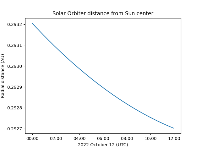
We can request the location of the spacecraft in any SPICE frame. Here, we request it in ‘SOLO_HEEQ’, which is Stonyhurst heliographic coordinates.

spacecraft = spice.get_body('Solar Orbiter', obstime, spice_frame='SOLO_HEEQ')
print(spacecraft[:4])

<SkyCoord (spice_SOLO_HEEQ: obstime=['2022-10-12T00:00:00.000' '2022-10-12T00:01:00.000'
 '2022-10-12T00:02:00.000' '2022-10-12T00:03:00.000']): (lon, lat, distance) in (deg, deg, km)
    [(-119.01442874, -3.70146927, 43862837.4129893 ),
     (-119.00981929, -3.70081081, 43862685.54244631),
     (-119.00520982, -3.70015232, 43862533.80289252),
     (-119.00060031, -3.6994938 , 43862382.1943316 )]>

Plot the radial distance from the Sun over the time range.

fig = plt.figure()
ax = fig.add_subplot()
ax.plot(obstime.datetime64, spacecraft.distance.to('AU'))
ax.xaxis.set_major_formatter(DateFormatter('%H:%M'))
ax.set_xlabel('2022 October 12 (UTC)')
ax.set_ylabel('Radial distance (AU)')
ax.set_title('Solar Orbiter distance from Sun center')

Text(0.5, 1.0, 'Solar Orbiter distance from Sun center')

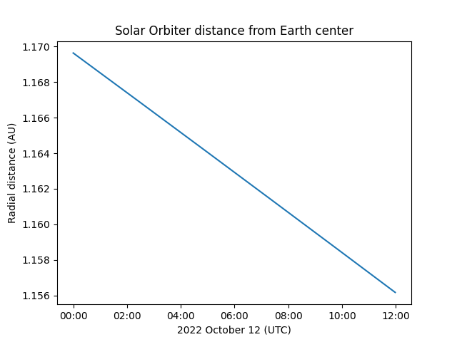
We can then transform the coordinate to a different SPICE frame. When specifying the frame for SkyCoord, SPICE frame names should be prepended with 'spice_'. Here, we transform it to ‘SOLO_GAE’.

spacecraft_gae = spacecraft.transform_to("spice_SOLO_GAE")
print(spacecraft_gae[:4])

<SkyCoord (spice_SOLO_GAE: obstime=['2022-10-12T00:00:00.000' '2022-10-12T00:01:00.000'
 '2022-10-12T00:02:00.000' '2022-10-12T00:03:00.000']): (lon, lat, distance) in (deg, deg, km)
    [(-149.06635464, -1.03769419, 1.74975667e+08),
     (-149.06492567, -1.03771064, 1.74972891e+08),
     (-149.0634967 , -1.03772709, 1.74970116e+08),
     (-149.06206775, -1.03774353, 1.74967339e+08)]>

Plot the radial distance from the Earth over the time range.

fig = plt.figure()
ax = fig.add_subplot()
ax.plot(obstime.datetime64, spacecraft_gae.distance.to('AU'))
ax.xaxis.set_major_formatter(DateFormatter('%H:%M'))
ax.set_xlabel('2022 October 12 (UTC)')
ax.set_ylabel('Radial distance (AU)')
ax.set_title('Solar Orbiter distance from Earth center')

Text(0.5, 1.0, 'Solar Orbiter distance from Earth center')

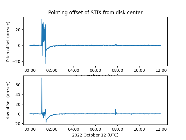
We can also leverage the Solar Orbiter SPICE kernels to look at instrument pointing. Let’s define a coordinate that points directly along the line of sight of the STIX instrument. For the ‘SOLO_STIX_ILS’ frame, 0 degrees longitude is in the anti-Sun direction, while 180 degrees longitude is in the Sun direction.

stix_ils = SkyCoord(np.repeat(0*u.deg, len(obstime)),
                    np.repeat(0*u.deg, len(obstime)),
                    frame='spice_SOLO_STIX_ILS', obstime=obstime)
print(stix_ils[:4])

<SkyCoord (spice_SOLO_STIX_ILS: obstime=['2022-10-12T00:00:00.000' '2022-10-12T00:01:00.000'
 '2022-10-12T00:02:00.000' '2022-10-12T00:03:00.000']): (lon, lat) in deg
    [(0., 0.), (0., 0.), (0., 0.), (0., 0.)]>

We can transform that line of sight to the SPICE frame ‘SOLO_SUN_RTN’, which is similar to helioprojective coordinates as observed from Solar Orbiter, except that the disk center is at 180 degrees longitude instead of 0 degrees longitude. Given how the line-of-sight coordinate is defined above, the latitude and longitude values of the resulting coordinate are the pitch and yaw offsets from disk center, respectively.

stix_ils_rtn = stix_ils.transform_to("spice_SOLO_SUN_RTN")
print(stix_ils_rtn[:4])

<SkyCoord (spice_SOLO_SUN_RTN: obstime=['2022-10-12T00:00:00.000' '2022-10-12T00:01:00.000'
 '2022-10-12T00:02:00.000' '2022-10-12T00:03:00.000']): (lon, lat) in deg
    [( 4.39902611e-05, -9.64402100e-06),
     (-6.15907476e-06,  3.35635709e-05),
     ( 7.84514218e-05,  5.45216843e-05),
     ( 1.38832795e-04, -2.82247275e-05)]>

Plot the pitch/yaw offsets over the time range.

fig, ax = plt.subplots(2, 1)
ax[0].plot(obstime.datetime64, stix_ils_rtn.lat.to('arcsec'))
ax[0].xaxis.set_major_formatter(DateFormatter('%H:%M'))
ax[0].set_xlabel('2022 October 12 (UTC)')
ax[0].set_ylabel('Pitch offset (arcsec)')
ax[1].plot(obstime.datetime64, stix_ils_rtn.lon.to('arcsec'))
ax[1].xaxis.set_major_formatter(DateFormatter('%H:%M'))
ax[1].set_xlabel('2022 October 12 (UTC)')
ax[1].set_ylabel('Yaw offset (arcsec)')
ax[0].set_title('Pointing offset of STIX from disk center')

plt.show()

Finally, we can query the instrument field of view (FOV) via SPICE, which will be in the ‘SOLO_STIX_ILS’ frame. This call returns the corners of the rectangular FOV of the STIX instrument, and you can see they are centered around 180 degrees longitude, which is the direction of the Sun in this frame.

stix_fov = spice.get_fov('SOLO_STIX', obstime[0])
print(stix_fov)

<SkyCoord (spice_SOLO_STIX_ILS: obstime=2022-10-12T00:00:00.000): (lon, lat) in deg
    [( 179.,  0.99984773), ( 179., -0.99984773), (-179., -0.99984773),
     (-179.,  0.99984773)]>

More usefully, every coordinate in a SPICE frame has a to_helioprojective() method that converts the coordinate to Helioprojective with the observer at the center of te SPICE frame. For the ‘SOLO_STIX_ILS’ frame, the center is Solar Orbiter, which is exactly what we want.

print(stix_fov.to_helioprojective())

<SkyCoord (Helioprojective: obstime=2022-10-12T00:00:00.000, rsun=695700.0 km, observer=<HeliographicStonyhurst Coordinate (obstime=2022-10-12T00:00:00.000, rsun=695700.0 km): (lon, lat, radius) in (deg, deg, km)
    (-119.01442835, -3.70146957, 43862838.51789755)>): (Tx, Ty) in arcsec
    [( 3127.44366521,  4016.7597387 ), ( 4017.02833491, -3126.974253  ),
     (-3127.76037459, -4016.69030973), (-4017.34508529,  3127.04367678)]>

🏷 Tags: Coordinates, Parker Solar Probe, Solar Orbiter