Masking HMI based on the intensity of AIA

In this example we will demonstrate how to mask out regions within a HMI image based on the intensity values of AIA.

import matplotlib.pyplot as plt
import numpy as np
from matplotlib.colors import Normalize
from skimage.measure import label, regionprops

import astropy.units as u
from astropy.coordinates import SkyCoord

import sunpy.map
from sunpy.data.sample import AIA_171_IMAGE, HMI_LOS_IMAGE

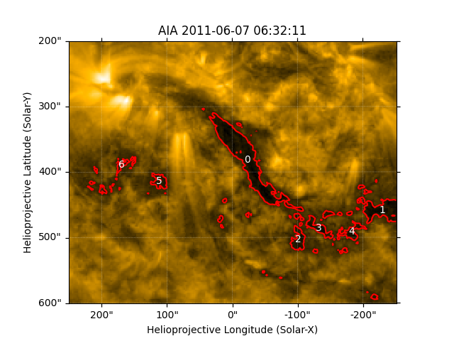
We will use an AIA 171 image from the sample data and crop it to capture a region of interest.

aia = sunpy.map.Map(AIA_171_IMAGE)
aia = aia.submap(
    bottom_left=SkyCoord(-250, 200, unit=u.arcsec, frame=aia.coordinate_frame),
    width=500 * u.arcsec,
    height=400 * u.arcsec,
)

Next we create the HMI map and crop it to the same field of view as the AIA image.

hmi = sunpy.map.Map(HMI_LOS_IMAGE)
hmi = hmi.submap(aia.bottom_left_coord, top_right=aia.top_right_coord)

We then call the reproject_to() to reproject the AIA Map to have exactly the same grid as the HMI Map. We choose to reproject the AIA data to the HMI grid, rather than the reverse, to avoid interpolating the LOS HMI magnetic field data. This is because the range of the HMI data includes both positive and negative values and interpolation can destroy small scale variations in the LOS magnetic field which may be important in some scientific contexts.

aia = aia.reproject_to(hmi.wcs)
aia.nickname = 'AIA'

Now we will identify separate regions below a threshold in the AIA Map. In this case, we want the darker patches that have pixel values below 200. Then, using skimage, we can label() and calculate the properties of each region using regionprops().

segmented = aia.data < 200
labeled = label(segmented)
regions = regionprops(labeled, hmi.data)
# We want the largest region, so we will sort by descending order in size.
regions = sorted(regions, key=lambda r: r.area, reverse=True)

Now to plot and label the first 7 regions seen in AIA with the region “0” being the largest.

fig = plt.figure()
ax = fig.add_subplot(projection=aia)
aia.plot(axes=ax)
aia.draw_contours(axes=ax, levels=200, colors="r")
for i in range(7):
    plt.text(*np.flip(regions[i].centroid), str(i), color="w", ha="center", va="center")

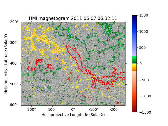
Now let’s plot those same regions on the HMI Map.

fig = plt.figure()
ax = fig.add_subplot(projection=hmi)
im = hmi.plot(axes=ax, cmap="hmimag", norm=Normalize(-1500, 1500))
aia.draw_contours(axes=ax, levels=200, colors="r")
fig.colorbar(im)

<matplotlib.colorbar.Colorbar object at 0x7f4548a63c10>

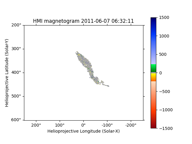
Now we have the regions, we need to create a new HMI map that masks out everything but the largest region. To do so, we need to create the mask from the bounding box returned by skimage. Note that we can do this from the thresholded region only because our AIA and HMI images are on the same pixel grid after reprojecting the AIA image.

bbox = regions[0].bbox
mask = np.ones_like(hmi.data, dtype=bool)
mask[bbox[0]: bbox[2], bbox[1]: bbox[3]] = ~regions[0].image
hmi_masked = sunpy.map.Map((hmi.data, hmi.meta), mask=mask)

We can then plot the largest HMI region.

fig = plt.figure()
ax = fig.add_subplot(projection=hmi_masked)
im = hmi_masked.plot(axes=ax, cmap="hmimag", norm=Normalize(-1500, 1500))
fig.colorbar(im)

<matplotlib.colorbar.Colorbar object at 0x7f4549198a30>

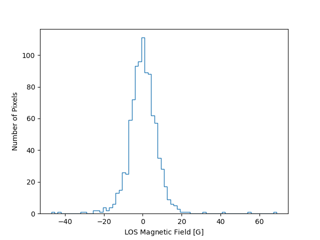
Finally, we can plot the distribution of HMI LOS magnetic field for only the unmasked values in the largest region shown above.

fig = plt.figure()
ax = fig.add_subplot()
ax.hist(hmi_masked.data[~hmi_masked.mask], bins='auto', histtype='step')
ax.set_ylabel('Number of Pixels')
ax.set_xlabel(f'LOS Magnetic Field [{hmi.unit:latex_inline}]')

plt.show()