Plotting Fields of View of Solar Orbiter and DKIST

In this example, we plot the fields of view of multiple Solar Orbiter instruments, alongside coordinated DKIST observations. These observations were taken during the Long-Term Active Region SOOP (R_SMALL_MRES_MCAD_AR-Long-Term).

import dkist.net  # NOQA: F401
import matplotlib.pyplot as plt
import numpy as np
from ndcube import NDCube

import astropy.units as u
from astropy.coordinates import SkyCoord
from astropy.io import fits
from astropy.wcs import WCS

import sunpy.map
from sunpy.net import Fido
from sunpy.net import attrs as a
from sunpy.visualization import drawing

INFO: Fetching updated search values for the DKIST client to /home/docs/.local/share/dkist/api_search_values.json [dkist.net.attrs_values]

Download and Read Multiple Observations

The first step is to search for and download multiple datasets. During this time window a coordinated campaign between Solar Orbiter and DKIST was underway.

time_range = a.Time("2022-10-24T18:55", "2022-10-24T19:35")

We search for EUI Full Sun Imager, EUI High Resolution Imager and SPICE data,

solo = (
    a.soar.Product("EUI-HRIEUV174-IMAGE") | a.soar.Product("EUI-FSI174-IMAGE") | a.soar.Product("SPICE-N-RAS")
) & a.Level(2)

as well as AIA 17.1 nm data,

aia = a.Instrument.aia & a.Wavelength(171 * u.Angstrom) & a.Sample(10 * u.minute)

and finally DKIST VBI and VISP data.

dkist_visp = a.Instrument.visp

dkist_vbi = a.Instrument.vbi & a.Wavelength(430 * u.nm, 431 * u.nm)

We combine all these searches using the | (or) operator and the time range.

results = Fido.search(
    time_range,
    solo | aia | dkist_vbi | dkist_visp,
)
print(results[:, 0])

Results from 6 Providers:

1 Results from the SOARClient:

Instrument     Data product    Level        Start time               End time        Filesize           SOOP Name            Detector Wavelength
                                                                                      Mbyte
---------- ------------------- ----- ----------------------- ----------------------- -------- ------------------------------ -------- ----------
       EUI eui-hrieuv174-image    L2 2022-10-24 19:00:00.171 2022-10-24 19:00:01.821    5.731 R_SMALL_MRES_MCAD_AR-Long-Term  HRI_EUV      174.0

1 Results from the SOARClient:

Instrument   Data product   Level        Start time               End time        Filesize           SOOP Name            Detector Wavelength
                                                                                   Mbyte
---------- ---------------- ----- ----------------------- ----------------------- -------- ------------------------------ -------- ----------
       EUI eui-fsi174-image    L2 2022-10-24 19:00:50.195 2022-10-24 19:01:00.195    4.697 R_SMALL_MRES_MCAD_AR-Long-Term      FSI      174.0

1 Results from the SOARClient:

Instrument Data product Level        Start time               End time        Filesize           SOOP Name            Detector Wavelength
                                                                               Mbyte
---------- ------------ ----- ----------------------- ----------------------- -------- ------------------------------ -------- ----------
     SPICE  spice-n-ras    L2 2022-10-24 19:01:34.618 2022-10-24 19:12:53.014  175.582 R_SMALL_MRES_MCAD_AR-Long-Term       SW       None

1 Results from the VSOClient:
Source: https://sdac.virtualsolar.org/cgi/search
Data retrieval status: http://docs.virtualsolar.org/wiki/VSOHealthReport
Total estimated size: 67.789 Mbyte

       Start Time               End Time        Source Instrument   Wavelength   Provider  Physobs  Wavetype Extent Width Extent Length Extent Type   Size
                                                                     Angstrom                                                                        Mibyte
----------------------- ----------------------- ------ ---------- -------------- -------- --------- -------- ------------ ------------- ----------- --------
2022-10-24 18:55:09.000 2022-10-24 18:55:10.000    SDO        AIA 171.0 .. 171.0     JSOC intensity   NARROW         4096          4096    FULLDISK 64.64844

1 Results from the DKISTClient:


Showing 1 of 2 available results.
Use a.dkist.Page(2) to show the second page of results.

Product ID Dataset ID        Start Time               End Time        Instrument   Wavelength
                                                                                       nm
---------- ---------- ----------------------- ----------------------- ---------- --------------
  L1-NAWGB     XYLAZY 2022-10-24T18:58:12.753 2022-10-24T18:58:37.127        VBI 430.0 .. 430.0

1 Results from the DKISTClient:

Product ID Dataset ID        Start Time               End Time        Instrument               Wavelength
                                                                                                   nm
---------- ---------- ----------------------- ----------------------- ---------- -------------------------------------
  L1-CEIIM      BKEWK 2022-10-24T18:57:45.634 2022-10-24T19:33:26.865       VISP 630.2424776472172 .. 631.826964866207

We will then just download the first results for all our different data sources.

files = Fido.fetch(results[:, 0], site="NSO")

# Sort the files by filename, but lowercase
files.sort(key=str.lower)

# Put the file paths into a dict
files = {name: path for name, path in zip(["AIA", "EUI-FSI", "EUI-HRI", "SPICE", "VBI", "VISP"], files)}

Open the images as sunpy maps

aia, eui_fsi, eui_hri = sunpy.map.Map(files["AIA"], files["EUI-FSI"], files["EUI-HRI"])

Load the SPICE file into a NDCube

hdul = fits.open(files["SPICE"])
hdu = hdul["N IV 765 - SH - Comp 8 ... Ne VIII 770 - LH - Comp 8 (Merged)"]

spice = NDCube(
    hdu.data,
    wcs=WCS(hdu),
    unit=hdu.header["BUNIT"],
    mask=np.isnan(hdu.data),
)

# Drop the length one time / raster repeat dimension
spice = spice.squeeze()

/home/docs/checkouts/readthedocs.org/user_builds/sunpy/conda/latest/lib/python3.13/site-packages/astropy/wcs/wcs.py:648: FITSFixedWarning: CROTA = 4.81035026522 / [deg] S/C counter-clockwise roll rel to Solar N
keyword looks very much like CROTAn but isn't.
  wcsprm = Wcsprm(
/home/docs/checkouts/readthedocs.org/user_builds/sunpy/conda/latest/lib/python3.13/site-packages/astropy/wcs/wcs.py:918: FITSFixedWarning: 'datfix' made the change 'Set MJDREF to 59876.792762 from DATEREF.
Set MJD-OBS to 59876.792762 from DATE-OBS.
Set MJD-BEG to 59876.792762 from DATE-BEG.
Set MJD-AVG to 59876.796688 from DATE-AVG.
Set MJD-END to 59876.800610 from DATE-END'.
  warnings.warn(

We then create a second cube which is summed across all wavelengths. This gives us a spatial only cube to use for extent calculations later.

spice_wl_sum = spice.rebin((-1, 1, 1), operation=np.sum).squeeze()

Open the VBI and VISP ASDF files with the dkist package Note this has not downloaded any of the array data, but we do not need this for this example.

vbi = dkist.load_dataset(files["VBI"])
visp = dkist.load_dataset(files["VISP"])

In a similar manner to SPICE we need to create a spatial only cube. As this VISP dataset also has a stokes axis, we drop this first and then sum over wavelength.

visp_I = visp[0]
visp_I_wl_sum = visp_I.rebin((1, -1, 1), operation=np.sum).squeeze()

Initial Plots

fig = plt.figure()
ax = fig.add_subplot(projection=eui_fsi)
eui_fsi.plot(axes=ax)

<matplotlib.image.AxesImage object at 0x721a67d84f50>

We can see that the FSI image is a little zoomed out, so let’s crop it down to closer to the limb.

eui_fsi_zoom = eui_fsi.submap(
    bottom_left=SkyCoord(-3000, -3000, unit="arcsec", frame=eui_fsi.coordinate_frame),
    top_right=SkyCoord(3000, 3000, unit="arcsec", frame=eui_fsi.coordinate_frame),
)

We are going to make a number of plots with the extents of all these data overplotted, so we define a quick helper function to do this.

def overplot_extents(ax):
    # Add the HRI extent.
    eui_hri.draw_extent(axes=ax, label="EUI HRI", color="C1")

    # Add the SPICE extent using the `~sunpy.visualization.drawing.extent` function as the SPICE data is not a Map.
    drawing.extent(axes=ax, wcs=spice_wl_sum.wcs, color="C2", label="SPICE")

    # Add the VISP FOV, using the same helper function.
    visible, hidden = drawing.extent(ax, wcs=visp_I_wl_sum.wcs, color="C4")
    visible.set_label("VISP")

    # The VBI data is a mosaic of 9 images, so we iterate over all of them and draw the extent of each.
    for ds in vbi.flat:
        visible, hidden = drawing.extent(ax, ds.wcs, color="C5")

    # Only add the last one to the legend
    visible.set_label("VBI")

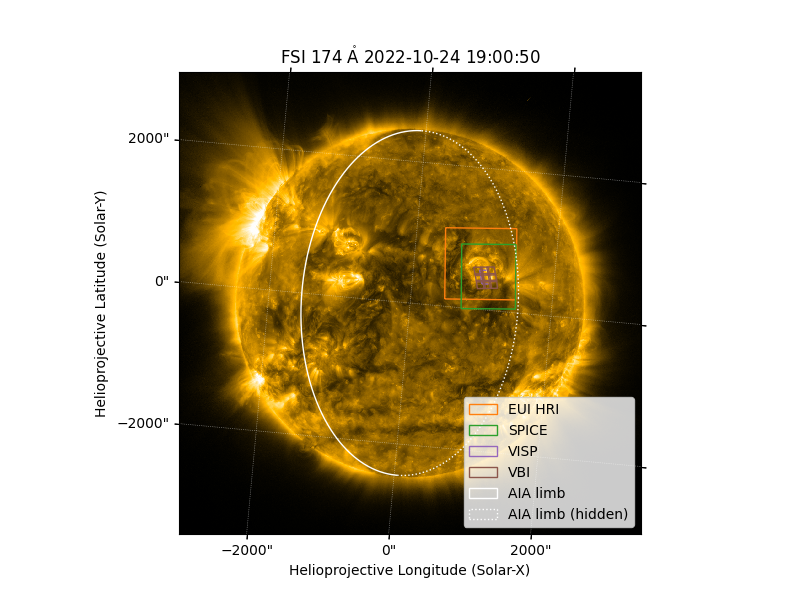
In this first plot we shall draw all the extents on top of the EUI FSI image, and add the AIA limb.

fig = plt.figure(figsize=(8, 6))
ax = fig.add_subplot(projection=eui_fsi_zoom)

# Plot the FSI image
eui_fsi_zoom.plot(axes=ax)

# Draw all extents
overplot_extents(ax)

# Add the AIA limb
visible, hidden = aia.draw_limb()
visible.set_label("AIA limb")
hidden.set_label("AIA limb (hidden)")

ax.legend()

/home/docs/checkouts/readthedocs.org/user_builds/sunpy/conda/latest/lib/python3.13/site-packages/erfa/core.py:16909: RuntimeWarning: invalid value encountered in taiutc
  utc1, utc2, c_retval = ufunc.taiutc(tai1, tai2)
/home/docs/checkouts/readthedocs.org/user_builds/sunpy/conda/latest/lib/python3.13/site-packages/erfa/core.py:133: ErfaWarning: ERFA function "taiutc" yielded 5112 of "dubious year (Note 4)"
  warn(f'ERFA function "{func_name}" yielded {wmsg}', ErfaWarning)

<matplotlib.legend.Legend object at 0x721a67df6850>

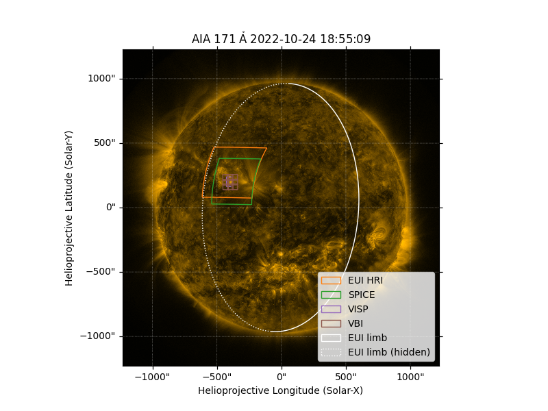
We shall now do the same but based on the AIA image.

fig = plt.figure(figsize=(8, 6))
ax = fig.add_subplot(projection=aia)

# Plot the AIA image
aia.plot(axes=ax)

# Draw all extents
overplot_extents(ax)

# Add the EUI FSI limb
visible, hidden = eui_fsi.draw_limb()
visible.set_label("EUI limb")
hidden.set_label("EUI limb (hidden)")

ax.legend()

/home/docs/checkouts/readthedocs.org/user_builds/sunpy/conda/latest/lib/python3.13/site-packages/erfa/core.py:16909: RuntimeWarning: invalid value encountered in taiutc
  utc1, utc2, c_retval = ufunc.taiutc(tai1, tai2)
/home/docs/checkouts/readthedocs.org/user_builds/sunpy/conda/latest/lib/python3.13/site-packages/erfa/core.py:133: ErfaWarning: ERFA function "taiutc" yielded 5112 of "dubious year (Note 4)"
  warn(f'ERFA function "{func_name}" yielded {wmsg}', ErfaWarning)

<matplotlib.legend.Legend object at 0x721a67d84050>

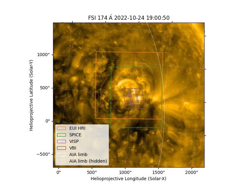
And finally let’s zoom in on the shared FOV

eui_fsi_crop = eui_fsi.submap(
    bottom_left=SkyCoord(-100, -500, unit="arcsec", frame=eui_fsi.coordinate_frame),
    top_right=SkyCoord(2000, 1500, unit="arcsec", frame=eui_fsi.coordinate_frame),
)

fig = plt.figure(figsize=(8, 6))
ax = fig.add_subplot(projection=eui_fsi_crop)
eui_fsi_crop.plot(axes=ax)

# Draw all extents
overplot_extents(ax)

# Add the AIA limb
visible, hidden = aia.draw_limb()
visible.set_label("AIA limb")
hidden.set_label("AIA limb (hidden)")

ax.legend()

plt.show()

/home/docs/checkouts/readthedocs.org/user_builds/sunpy/conda/latest/lib/python3.13/site-packages/erfa/core.py:16909: RuntimeWarning: invalid value encountered in taiutc
  utc1, utc2, c_retval = ufunc.taiutc(tai1, tai2)
/home/docs/checkouts/readthedocs.org/user_builds/sunpy/conda/latest/lib/python3.13/site-packages/erfa/core.py:133: ErfaWarning: ERFA function "taiutc" yielded 5112 of "dubious year (Note 4)"
  warn(f'ERFA function "{func_name}" yielded {wmsg}', ErfaWarning)

🏷 Tags: Coordinates, Solar Orbiter, Map, SOAR, EUI, SPICE, AIA, DKIST, VBI, VISP, Visualization