Note
Go to the end to download the full example code.
Overplotting HMI Contours on an AIA Image#
This example shows how to use wcsaxes to overplot
unaligned HMI magnetic field strength contours on an AIA map.
import matplotlib.pyplot as plt
import numpy as np

import astropy.units as u
from astropy.coordinates import SkyCoord

import sunpy.map
from sunpy.data.sample import AIA_193_IMAGE, HMI_LOS_IMAGE
First let’s load two of the sample files into two Map objects.
aia, hmi = sunpy.map.Map(AIA_193_IMAGE, HMI_LOS_IMAGE)
To make the plot neater, we start by submapping the same region. We define the region in HGS coordinates and then apply the same submap to both the HMI and AIA maps.
bottom_left = SkyCoord(30 * u.deg, -40 * u.deg, frame='heliographic_stonyhurst')
top_right = SkyCoord(70 * u.deg, 0 * u.deg, frame='heliographic_stonyhurst')

sub_aia = aia.submap(bottom_left, top_right=top_right)
sub_hmi = hmi.submap(bottom_left, top_right=top_right)
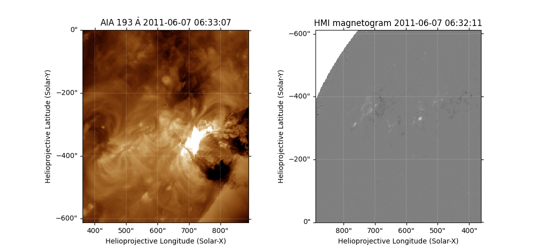
To highlight the fact that the AIA and HMI images are not aligned, let us quickly view the two maps side-by-side.
fig = plt.figure(figsize=(11, 5))

ax1 = fig.add_subplot(121, projection=sub_aia)
sub_aia.plot(axes=ax1, clip_interval=(1, 99.99)*u.percent)

ax2 = fig.add_subplot(122, projection=sub_hmi)
sub_hmi.plot(axes=ax2)
<matplotlib.image.AxesImage object at 0x744fc4579450>
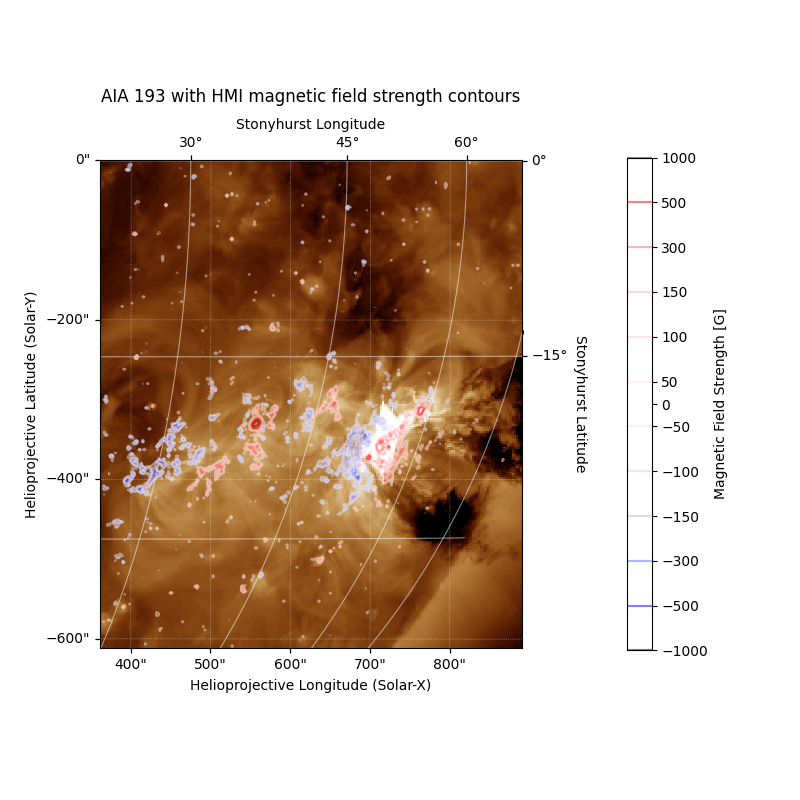
In the next plot we will start by plotting the same aia submap, and draw a heliographic grid on top.
fig = plt.figure(figsize=(8, 8))

ax = fig.add_subplot(projection=sub_aia)
sub_aia.plot(axes=ax, clip_interval=(1, 99.99)*u.percent)
sub_aia.draw_grid(axes=ax)

ax.set_title("AIA 193 with HMI magnetic field strength contours", y=1.1)
Text(0.5, 1.1, 'AIA 193 with HMI magnetic field strength contours')
Now we want to draw the contours, to enhance the appearance of the plot we explicitly list the levels, but then make them symmetric around 0
matplotlib requires the levels to be sorted, so we order them from lowest to highest by reversing the array.
levels = np.concatenate((-1 * levels[::-1], levels))
Before we add the contours to the axis we store the existing bounds of the as overplotting the contours will sometimes change the bounds, we re-apply them to the axis after the contours have been added.
We use the map method draw_contours to simplify this process,
but this is a wrapper around contour. We set the
colormap, line width and transparency of the lines to improve the final
appearance.
(np.float64(-0.5), np.float64(219.5), np.float64(-0.5), np.float64(254.5))
Finally, add a colorbar. We add an extra tick to the colorbar at the 0 point to make it clearer that it is symmetric, and tweak the size and location to fit with the axis better.
plt.colorbar(cset,
             label=f"Magnetic Field Strength [{sub_hmi.unit}]",
             ticks=list(levels.value) + [0],
             shrink=0.8,
             pad=0.17)

plt.show()
Total running time of the script: (0 minutes 0.848 seconds)