Downloading and plotting Metis coronagraph data

This example demonstrates how to download, load, and visualize visible-light total brightness observations from the Metis coronagraph aboard the Solar Orbiter mission.

Metis observes the solar corona by occulting the bright solar disk, allowing faint coronal structures to be imaged in visible light and ultraviolet wavelengths.

import matplotlib.pyplot as plt
import numpy as np
from matplotlib import colors

import astropy.units as u

import sunpy.map
from sunpy.net import Fido
from sunpy.net import attrs as a

The Metis instrument provides visible-light (VL) and ultraviolet (UV) data products. In this example we will demonstrate the plotting of the VL total-brightness data product. We first plot a single map, and then build a MapSequence to animate a coronal eruption as a running-difference movie. In the second example we will showcase the UV data and helpful operations

The data is served by the Solar Orbiter Archive (SOAR), so we set a.Provider.soar. Here we query for the Level 2, visible-light total-brightness product (a.soar.Product.metis_vl_tb) over a time range covering an eruption event.

vl_result = Fido.search(a.Time("2022-03-22 21:00", "2022-03-22 22:50"),
                     a.Instrument.metis, a.Level(2), a.Provider.soar,
                     a.soar.Product.metis_vl_tb)
metis_files = Fido.fetch(vl_result)

The downloaded Metis fits file contains multiple image header data units (HDUs). When passed to Map, SunPy creates a MapSequence containing one map for each HDU. We then filter the sequence to obtain only the VL total-brightness maps. Finally, we select the first VL total-brightness map.

vl_maps = sunpy.map.Map(metis_files[0])
vl_tb_list = [m for m in vl_maps if m.measurement == "VL-TB"]
vl_tb_example = vl_tb_list[0]

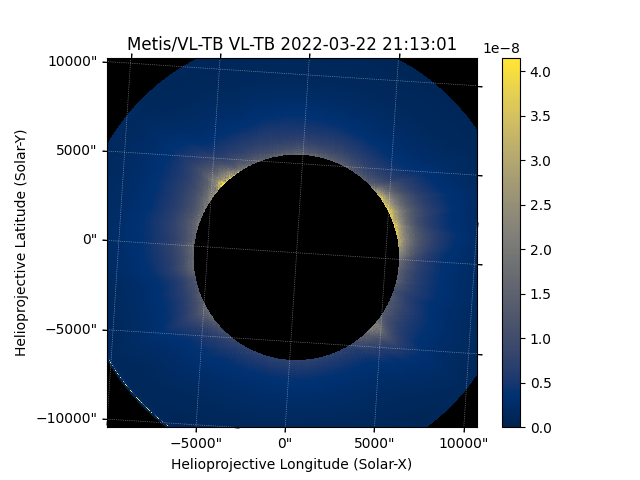
A METISMap is created with a default mask property that # flags pixels inside the inner occulter and outside the outer field of view. When the METISMap is plotted, the masked # pixels are not shown, so only the annular region observed by the coronagraph is visible.

fig = plt.figure()
ax = fig.add_subplot(projection=vl_tb_example)
im = vl_tb_example.plot(axes=ax)
fig.colorbar(im)

<matplotlib.colorbar.Colorbar object at 0x762f74178050>

In this example, the observation captured an eruption event. To visualise this, we build a time series sequence of maps and animate it. We load all of the downloaded files at once (again getting a list of maps), keep just the VL-TB maps, and combine them into a MapSequence by passing sequence=True

vl_tb_maps = sunpy.map.Map(metis_files)
m_seq_vltb = sunpy.map.Map([m for m in vl_tb_maps if m.measurement == "VL-TB"], sequence=True)

To get a better idea of what the event looks like we need to create a running difference.

m_seq_running = sunpy.map.Map(
    [m - prev_m.quantity for m, prev_m in zip(m_seq_vltb[1:], m_seq_vltb[:-1])],
    sequence=True
)

/home/docs/checkouts/readthedocs.org/user_builds/sunpy/conda/latest/lib/python3.13/site-packages/sunpy/map/mapbase.py:804: SunpyMetadataWarning: Could not parse unit string "MSB" as a valid FITS unit.
See https://docs.sunpy.org/en/stable/how_to/fix_map_metadata.html for how to fix metadata before loading it with sunpy.map.Map.
See https://fits.gsfc.nasa.gov/fits_standard.html for the FITS unit standards.
  warn_metadata(f'Could not parse unit string "{unit_str}" as a valid FITS unit.\n'
/home/docs/checkouts/readthedocs.org/user_builds/sunpy/conda/latest/lib/python3.13/site-packages/sunpy/map/mapbase.py:804: SunpyMetadataWarning: Could not parse unit string "MSB" as a valid FITS unit.
See https://docs.sunpy.org/en/stable/how_to/fix_map_metadata.html for how to fix metadata before loading it with sunpy.map.Map.
See https://fits.gsfc.nasa.gov/fits_standard.html for the FITS unit standards.
  warn_metadata(f'Could not parse unit string "{unit_str}" as a valid FITS unit.\n'
/home/docs/checkouts/readthedocs.org/user_builds/sunpy/conda/latest/lib/python3.13/site-packages/sunpy/map/mapbase.py:804: SunpyMetadataWarning: Could not parse unit string "MSB" as a valid FITS unit.
See https://docs.sunpy.org/en/stable/how_to/fix_map_metadata.html for how to fix metadata before loading it with sunpy.map.Map.
See https://fits.gsfc.nasa.gov/fits_standard.html for the FITS unit standards.
  warn_metadata(f'Could not parse unit string "{unit_str}" as a valid FITS unit.\n'
/home/docs/checkouts/readthedocs.org/user_builds/sunpy/conda/latest/lib/python3.13/site-packages/sunpy/map/mapbase.py:804: SunpyMetadataWarning: Could not parse unit string "MSB" as a valid FITS unit.
See https://docs.sunpy.org/en/stable/how_to/fix_map_metadata.html for how to fix metadata before loading it with sunpy.map.Map.
See https://fits.gsfc.nasa.gov/fits_standard.html for the FITS unit standards.
  warn_metadata(f'Could not parse unit string "{unit_str}" as a valid FITS unit.\n'
/home/docs/checkouts/readthedocs.org/user_builds/sunpy/conda/latest/lib/python3.13/site-packages/sunpy/map/mapbase.py:804: SunpyMetadataWarning: Could not parse unit string "MSB" as a valid FITS unit.
See https://docs.sunpy.org/en/stable/how_to/fix_map_metadata.html for how to fix metadata before loading it with sunpy.map.Map.
See https://fits.gsfc.nasa.gov/fits_standard.html for the FITS unit standards.
  warn_metadata(f'Could not parse unit string "{unit_str}" as a valid FITS unit.\n'
/home/docs/checkouts/readthedocs.org/user_builds/sunpy/conda/latest/lib/python3.13/site-packages/sunpy/map/mapbase.py:804: SunpyMetadataWarning: Could not parse unit string "MSB" as a valid FITS unit.
See https://docs.sunpy.org/en/stable/how_to/fix_map_metadata.html for how to fix metadata before loading it with sunpy.map.Map.
See https://fits.gsfc.nasa.gov/fits_standard.html for the FITS unit standards.
  warn_metadata(f'Could not parse unit string "{unit_str}" as a valid FITS unit.\n'

Now we can normalise the values from all the maps and create a running difference animation

all_diff_data = np.concatenate([m.data for m in m_seq_running])
vmin, vmax = np.percentile(all_diff_data, [0.05, 99.95])
norm = colors.Normalize(vmin=vmin, vmax=vmax)

fig = plt.figure()
ax = fig.add_subplot(projection=m_seq_running.maps[0])
ani_running = m_seq_running.plot(
    axes=ax,
    title='VL-TB Running Difference',
    norm=norm
)
plt.colorbar(extend='both', label=m_seq_running[0].unit.to_string())
plt.show()

Once Loop Reflect

Now we move on to the UV data product. First, let’s search for and download a Metis UV observation from SOAR.

uv_result = Fido.search(
    a.Time("2024-12-09 00:36", "2024-12-09 00:38"),
    a.Instrument.metis,
    a.Level(2),
    a.Provider.soar,
    a.soar.Product.metis_uv_image,
)
metis_uv_file = Fido.fetch(uv_result)

As with the VL product, the UV file stores several products as separate image HDUs, so Map again returns a list of maps. We keep just the UV intensity maps (measurement == "UV") and select the first one.

metis_uv_data = sunpy.map.Map(metis_uv_file[0])
metis_map = metis_uv_data[0]

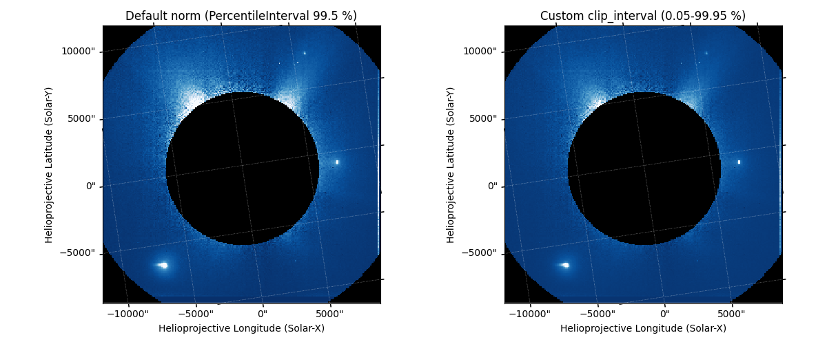
By default, METISMap sets a norm using PercentileInterval at 99.5 %. For data with a wide dynamic range this is often a good starting point, but you can tighten or loosen it by updating the norm’s interval directly, or by passing norm=None and using clip_interval to build a fresh norm from a chosen percentile range.

fig, axes = plt.subplots(1, 2, subplot_kw={"projection": metis_map},
                         figsize=(12, 5))

# Left panel: default plot_settings norm
metis_map.plot(axes=axes[0], cmap=metis_map.plot_settings["cmap"])
axes[0].set_title("Default norm (PercentileInterval 99.5 %)")

# Right panel: norm=None lets clip_interval take over
metis_map.plot(
    axes=axes[1],
    cmap=metis_map.plot_settings["cmap"],
    norm=None,
    clip_interval=(0.05, 99.95) * u.percent,
)
axes[1].set_title("Custom clip_interval (0.05-99.95 %)")

plt.tight_layout()
plt.show()

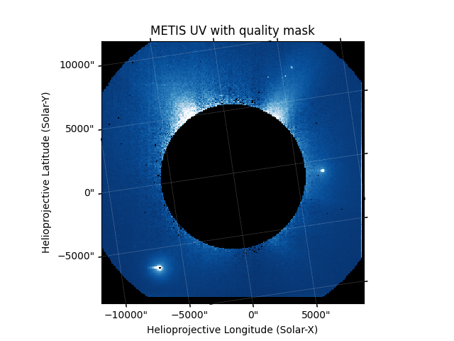
The UV data can contain a small number of very bright outlier pixels. We can flag them by using the quality mask from Metis file that is provided in the second map of the HDUs and merge it with the map’s existing occulter mask.

qmat = metis_uv_data[1].data
metis_map.mask = metis_map.mask | ~qmat.astype(bool)

fig = plt.figure()
ax = fig.add_subplot(projection=metis_map)
im = metis_map.plot(axes=ax)
ax.set_title("METIS UV with quality mask")
plt.show()

🏷 Tags: Map, Metis, SOAR, Solar Orbiter, Visualization