Note
Go to the end to download the full example code.
Create a Helioprojective Map from observations in the RA-DEC coordinate system#
How to create a Map in Helioprojective Coordinate Frame from radio observations
in GCRS (RA-DEC).
In this example a LOFAR FITS file (created with LOFAR’s Default Pre-Processing Pipeline (DPPP) and
WSClean Imager) is read in,
the WCS header information is then used to make a new header with the information in Helioprojective,
and a Map is made.
The LOFAR example file has a WCS in celestial coordinates i.e. Right Ascension and
Declination (RA-DEC). For this example, we are assuming that the definition of LOFAR’s
coordinate system for this observation is exactly the same as Astropy’s ~astropy.coordinates.GCRS.
For many solar studies we may want to plot this data in some Sun-centered coordinate frame,
such as Helioprojective. In this example we read the data and
header information from the LOFAR FITS file and then create a new header with updated WCS
information to create a Map with a HPC coordinate frame. We will make use of the
astropy.coordinates and sunpy.coordinates submodules together with
make_fitswcs_header() to create a new header and generate a
Map.
import matplotlib.pyplot as plt
import numpy as np

import astropy.units as u
from astropy.coordinates import EarthLocation, SkyCoord
from astropy.io import fits
from astropy.time import Time

import sunpy.data.sample
import sunpy.map
from sunpy.coordinates import frames, sun
We will first begin be reading in the header and data from the FITS file.
The data in this file is in a datacube structure to hold difference frequencies and polarizations. We are only interested in the image at one frequency (the only data in the file) so we index the data array to be the 2D data of interest.
We can inspect the header, for example, we can print the coordinate system and type projection, which here is RA-DEC.
RA---SIN DEC--SIN
Lets pull out the observation time and wavelength from the header, we will use these to create our new header.
To create a new Map header we need convert the reference coordinate
in RA-DEC (that is in the header) to Helioprojective. To do this we will first create
an astropy.coordinates.SkyCoord of the reference coordinate from the header information.
We will need the location of the observer (i.e. where the observation was taken).
We first establish the location on Earth from which the observation takes place, in this
case LOFAR observations are taken from Exloo in the Netherlands, which we define in lat and lon.
We can convert this to a SkyCoord in GCRSat the observation time.
lofar_loc = EarthLocation(lat=52.905329712*u.deg, lon=6.867996528*u.deg)
lofar_gcrs = SkyCoord(lofar_loc.get_gcrs(obstime))
We can then define the reference coordinate in terms of RA-DEC from the header information.
Here we are using the obsgeoloc keyword argument to take into account that the observer is not
at the center of the Earth (i.e. the GCRS origin). The distance here is the Sun-observer distance.
reference_coord = SkyCoord(header['crval1']*u.Unit(header['cunit1']),
                           header['crval2']*u.Unit(header['cunit2']),
                           frame='gcrs',
                           obstime=obstime,
                           obsgeoloc=lofar_gcrs.cartesian,
                           obsgeovel=lofar_gcrs.velocity.to_cartesian(),
                           distance=lofar_gcrs.hcrs.distance)
Now we can convert the reference_coord to the HPC coordinate frame.
Now we need to get the other parameters from the header that will be used to create the new header - here we can get the cdelt1 and cdelt2 which are the spatial scales of the data axes.
Finally, we need to specify the orientation of the HPC coordinate grid because
GCRS north is not in the same direction as HPC north. For convenience, we use
P() to calculate this relative rotation angle,
although due to subtleties in definitions, the returned value is inaccurate by
2 arcmin, equivalent to a worst-case shift of 0.6 arcsec for HPC coordinates
on the disk. The image will need to be rotated by this angle so that solar north
is pointing up.
Now we can use this information to create a new header using the helper
function make_fitswcs_header(). This will
create a MetaDict which will contain all the necessary WCS information to
create a Map. We provide a reference coordinate (in HPC),
the spatial scale of the observation (i.e., cdelt1 and cdelt2),
and the rotation angle (P1). Note that here, 1 is subtracted from the
crpix1 and crpix2 values, this is because the reference_pixel
keyword in :func:~sunpy.map.header_helper.make_fitswcs_header` is zero
indexed rather than the fits convention of 1 indexed.
new_header = sunpy.map.make_fitswcs_header(data, reference_coord_arcsec,
                                           reference_pixel=u.Quantity([header['crpix1']-1,
                                                                       header['crpix2']-1]*u.pixel),
                                           scale=u.Quantity([cdelt1, cdelt2]*u.arcsec/u.pix),
                                           rotation_angle=-P1,
                                           wavelength=frequency.to(u.MHz).round(2),
                                           observatory='LOFAR')
Let’s inspect the new header.
print(new_header)
('wcsaxes': '2')
('crpix1': '401.0')
('crpix2': '401.0')
('cdelt1': '20.000000000000018')
('cdelt2': '20.000000000000018')
('cunit1': 'arcsec')
('cunit2': 'arcsec')
('ctype1': 'HPLN-TAN')
('ctype2': 'HPLT-TAN')
('crval1': '2968.682862035918')
('crval2': '209.9412294598465')
('lonpole': '180.0')
('latpole': '0.0')
('mjdref': '0.0')
('date-obs': '2019-04-09T13:11:36.200')
('rsun_ref': '695700000.0')
('dsun_obs': '149822938834.19')
('hgln_obs': '-0.0013230706129548')
('hglt_obs': '-6.0483966759632')
('obsrvtry': 'LOFAR')
('wavelnth': '70.31')
('waveunit': 'MHz')
('naxis': '2')
('naxis1': '800')
('naxis2': '800')
('pc1_1': '0.8969123480105654')
('pc1_2': '-0.44220836715984285')
('pc2_1': '0.44220836715984285')
('pc2_2': '0.8969123480105654')
('rsun_obs': '957.7901922846717')
Lets create a Map.
lofar_map = sunpy.map.Map(data, new_header)
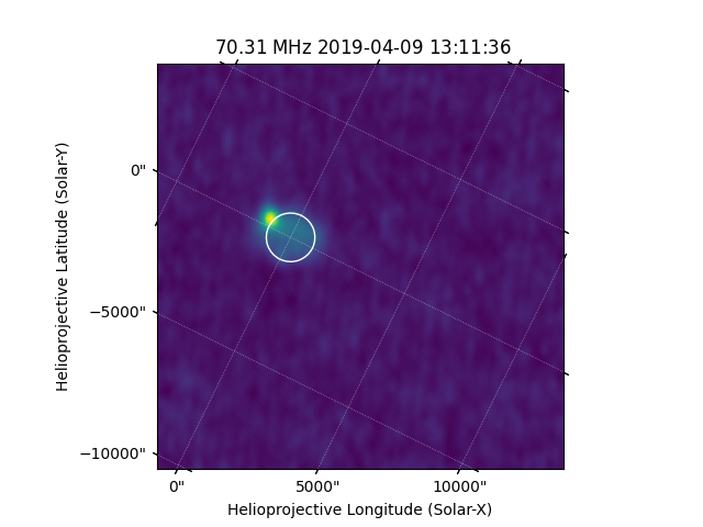
We can now plot this map and inspect it.
fig = plt.figure()
ax = fig.add_subplot(projection=lofar_map)
lofar_map.plot(axes=ax, cmap='viridis')
lofar_map.draw_limb(axes=ax)

plt.show()
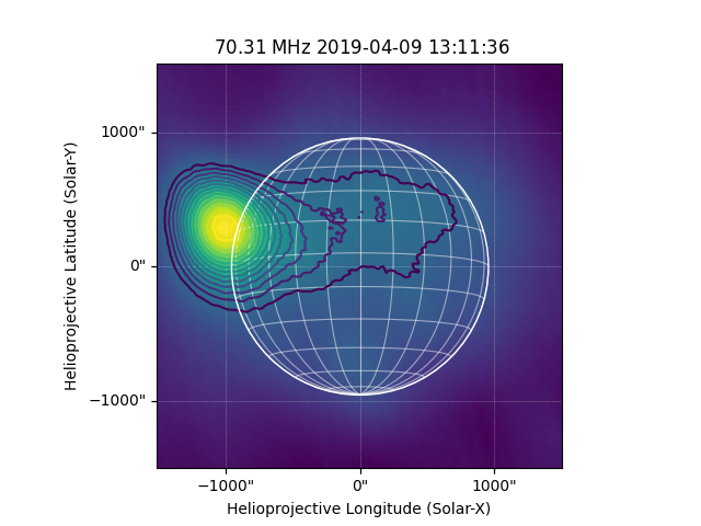
We can now rotate the image so that solar north is pointing up and create a submap in the field of view of interest.
Now lets plot this map, and overplot some contours.
Total running time of the script: (0 minutes 0.671 seconds)