Plotting a solar cycle index

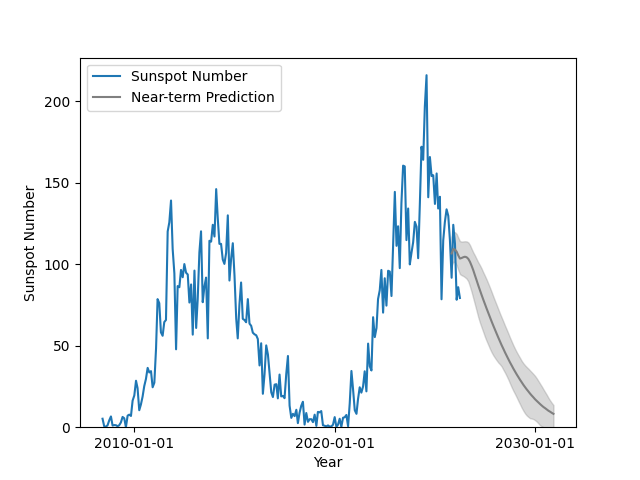
This example demonstrates how to plot the solar cycle in terms of the number of sunspots and a prediction for the next few years.

import matplotlib.pyplot as plt

import astropy.units as u
from astropy.time import Time, TimeDelta
from astropy.visualization import time_support

import sunpy.timeseries as ts
from sunpy.net import Fido
from sunpy.net import attrs as a
from sunpy.time import TimeRange

The U.S. Dept. of Commerce, NOAA, Space Weather Prediction Center (SWPC) provides recent solar cycle indices which includes different sunspot numbers, radio flux, and geomagnetic index. They also provide predictions for how the sunspot number and radio flux will evolve. Predicted values are based on the consensus of the Solar Cycle 24 Prediction Panel.

We will first search for and then download the data.

time_range = TimeRange("2008-06-01 00:00", Time.now())
result = Fido.search(a.Time(time_range), a.Instrument('noaa-indices'))
f_noaa_indices = Fido.fetch(result)
result = Fido.search(a.Time(time_range.end, time_range.end + TimeDelta(4 * u.year)),
                     a.Instrument('noaa-predict'))
f_noaa_predict = Fido.fetch(result)

We then load them into individual TimeSeries objects.

noaa = ts.TimeSeries(f_noaa_indices, source='noaaindices').truncate(time_range)
noaa_predict = ts.TimeSeries(f_noaa_predict, source='noaapredictindices')

Finally, we plot both noaa and noaa_predict for the sunspot number. In this case we use the S.I.D.C. Brussels International Sunspot Number (RI). The predictions provide both a high and low values, which we plot below as ranges.

time_support()
fig, ax = plt.subplots()
ax.plot(noaa.time, noaa.quantity('sunspot RI'), label='Sunspot Number')
ax.plot(
    noaa_predict.time, noaa_predict.quantity('sunspot'),
    color='grey', label='Near-term Prediction'
)
ax.fill_between(
    noaa_predict.time, noaa_predict.quantity('sunspot low'),
    noaa_predict.quantity('sunspot high'), alpha=0.3, color='grey'
)
ax.set_ylim(bottom=0)
ax.set_ylabel('Sunspot Number')
ax.set_xlabel('Year')
ax.legend()

plt.show()