Making a power spectrum from a TimeSeries

How to estimate the power spectrum of a TimeSeries.

import matplotlib.pyplot as plt
from scipy import signal

import astropy.units as u

import sunpy.timeseries
from sunpy.data.sample import RHESSI_TIMESERIES

Let’s first load a RHESSI TimeSeries from sunpy’s sample data. This data contains 9 columns, which are evenly sampled with a time step of 4 seconds.

ts = sunpy.timeseries.TimeSeries(RHESSI_TIMESERIES)

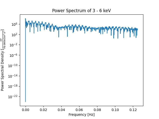
We now use SciPy’s periodogram to estimate the power spectra of the first column of the Timeseries. The first column contains X-Ray emissions in the range of 3-6 keV. An alternative version is Astropy’s LombScargle periodogram.

x_ray = ts.columns[0]
# The suitable value for fs would be 0.25 Hz as the time step is 4 s.
freq, spectra = signal.periodogram(ts.quantity(x_ray), fs=0.25)

Let’s plot the results.

fig, ax = plt.subplots()
ax.semilogy(freq, spectra)
ax.set_title(f'Power Spectrum of {x_ray}')
ax.set_ylabel(f'Power Spectral Density [{ts.units[x_ray] ** 2 / u.Hz:LaTeX}]')
ax.set_xlabel('Frequency [Hz]')
plt.show()