Finding bright regions with ndimage

How you can to find the brightest regions in an AIA image and count the approximate number of regions of interest using ndimage.

import matplotlib.pyplot as plt
from scipy import ndimage

import sunpy.map
from sunpy.data.sample import AIA_193_IMAGE

We start with the sample data.

aiamap_mask = sunpy.map.Map(AIA_193_IMAGE)
aiamap = sunpy.map.Map(AIA_193_IMAGE)

First we make a mask, which tells us which regions are bright. We choose the criterion that the data should be at least 10% of the maximum value. Pixels with intensity values greater than this are included in the mask, while all other pixels are excluded.

mask = aiamap.data < aiamap.max() * 0.10

Mask is a bool array. It can be used to modify the original map object without modifying the data. Once this mask attribute is set, we can plot the image again.

aiamap_mask.mask = mask

fig = plt.figure()
ax = fig.add_subplot(projection=aiamap_mask)
aiamap_mask.plot(axes=ax)
plt.colorbar()

plt.show()

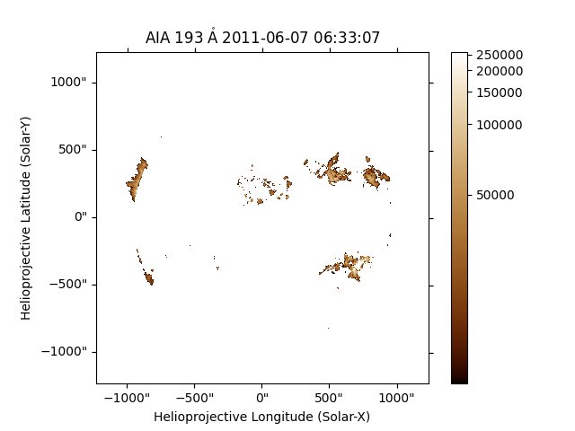
Only the brightest pixels remain in the image. However, these areas are artificially broken up into small regions. We can solve this by applying some smoothing to the image data. Here we apply a 2D Gaussian smoothing function to the data.

data2 = ndimage.gaussian_filter(aiamap.data * ~mask, 14)

The issue with the filtering is that it create pixels where the values are small (<100), so when we go on later to label this array, we get one large region which encompasses the entire array. If you want to see, just remove this line.

data2[data2 < 100] = 0

Now we will make a second sunpy map with this smoothed data.

aiamap2 = sunpy.map.Map(data2, aiamap.meta)

The function scipy.ndimage.label counts the number of contiguous regions in an image.

labels, n = ndimage.label(aiamap2.data)

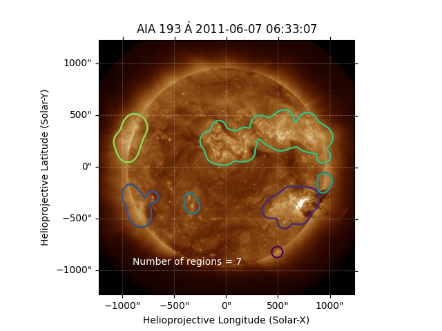
Finally, we plot the smoothed bright image data, along with the estimate of the number of distinct regions. We can see that approximately 6 distinct hot regions are present above the 10% of the maximum level.

fig = plt.figure()
ax = fig.add_subplot(projection=aiamap)
aiamap.plot(axes=ax)
ax.contour(labels)
plt.figtext(0.3, 0.2, f'Number of regions = {n}', color='white')

plt.show()