HXIMap#
- class sunpy.map.sources.HXIMap(data, header, **kwargs)[source]#
Bases:
GenericMapHXI Image Map Source.
The Hard X-ray Imager (HXI, Su et al. [2019], Zhang et al. [2019]) is one of the three payloads of the Advanced Space-based Solar Observatory (ASO-S, Gan et al. [2019], Gan et al. [2023]), which is designed to observe Hard X-Ray (HXR) spectra and images of solar flares. Having 91 subcollimators to modulate incident x-rays, HXI can obtain 91 modulation data and 45 visibilities to reconstruct images with a spatial resolution as high as ~3.1 arcsec.
In addition, the energy ranges are ~15-300 keV for imaging and ~10-300 keV for spectra, more information please refer to Su et al. [2024].
The HXI level 1 detector data, which is provided by the ASO-S Data Center, can be further processed by the HXI data analysis software to make hard X-ray images and export them as a FITS file. There may be more than one image included in the FITS file, from different time and energy intervals, which can be loaded by
Mapas a singleHXIMap(for one image) or alistcontaining multipleHXIMap.It is suggested to pay attention to the updates in the data and software versions, and feel free to contact the ASO-S/HXI team if there are any difficulties in data processing. Some useful links are attached in the references section below.
Notes
A number of the properties of this class are returned as two-value named tuples that can either be indexed by position ([0] or [1]) or be accessed by the names (.x and .y) or (.axis1 and .axis2). Things that refer to pixel axes use the
.x,.yconvention, where x and y refer to the FITS axes (x for columns y for rows). Spatial axes use.axis1and.axis2which correspond to the first and second axes in the header.axis1corresponds to the coordinate axis forxandaxis2corresponds toy.This class assumes that the metadata adheres to the FITS 4 standard. Where the CROTA2 metadata is provided (without PC_ij) it assumes a conversion to the standard PC_ij described in section 6.1 of Calabretta and Greisen [2002].
Warning
If a header has CD_ij values but no PC_ij values, CDELT values are required for this class to construct the WCS. If a file with more than two dimensions is feed into the class, only the first two dimensions (NAXIS1, NAXIS2) will be loaded and the rest will be discarded.
References
The tests and calibrations paper: Su et al. [2024]
Attributes Summary
The physical coordinate at the center of the bottom left ([0, 0]) pixel.
Observer Carrington latitude.
Observer Carrington longitude.
Return a coordinate object for the center pixel of the array.
Return the
matplotlib.colors.Colormapinstance this map uses.An
astropy.coordinates.BaseCoordinateFrameinstance created from the coordinate information for this Map, or None if the frame cannot be determined.Coordinate system used for x and y axes (ctype1/2).
The stored dataset.
The observation time.
Average time of the image acquisition.
Time of the end of the image acquisition.
DATE-OBS is the start_date.
Detector name.
The dimensions of the array (x axis first, y axis second).
Observer distance from the center of the Sun.
The
numpy.dtypeof the array of the map.Exposure time of the image.
A
Headerrepresentation of themetaattribute.Observer heliographic latitude.
Observer heliographic longitude.
Instrument name.
LaTeX formatted description of the Map.
Mask for the dataset, if any.
The measurement type of the observation.
Human-readable description of the Map.
The value of
numpy.ndarray.ndimof the data array of the map.An abbreviated human-readable description of the map-type; part of the Helioviewer data model.
Observatory or Telescope name.
The Heliographic Stonyhurst Coordinate of the observer.
Returns the FITS processing level if present.
Image representation of the PSF for the dataset.
Unitful representation of the map data.
Reference point WCS axes in data units (i.e. crval1, crval2).
The reference date for the coordinate system.
Pixel of reference coordinate.
Matrix describing the transformation needed to align the reference pixel with the coordinate axes.
Assumed radius of observed emission from the Sun center.
Angular radius of the observation from Sun center.
Image scale along the x and y axes in units/pixel (i.e. cdelt1, cdelt2).
Image coordinate units along the x and y axes (i.e. cunit1, cunit2).
The
Unitof the exposure time of this observation.The physical coordinate at the center of the the top right ([-1, -1]) pixel.
Uncertainty in the dataset, if any.
Unit of the map data.
Wavelength of the observation.
The
Unitof the wavelength of this observation.The
WCSproperty of the map.Methods Summary
draw_contours(levels[, axes, fill])Draw contours of the data.
draw_extent(*[, axes])Draw the extent of the map onto a given axes.
draw_grid([axes, grid_spacing, annotate, system])Draws a coordinate overlay on the plot in the Heliographic Stonyhurst coordinate system.
draw_limb([axes, resolution])Draws the solar limb as seen by the map's observer.
draw_quadrangle(bottom_left, *[, width, ...])Draw a quadrangle defined in world coordinates on the plot using Astropy's
Quadrangle.find_contours(level[, method])Returns coordinates of the contours for a given level value.
is_datasource_for(data, header, **kwargs)Determines if header corresponds to a HXI image.
max(*args, **kwargs)Calculate the maximum value of the data array, ignoring NaNs.
mean(*args, **kwargs)Calculate the mean of the data array, ignoring NaNs.
min(*args, **kwargs)Calculate the minimum value of the data array, ignoring NaNs.
peek([draw_limb, draw_grid, colorbar])Displays a graphical overview of the data in this object for user evaluation.
pixel_to_world(x, y)Convert a pixel coordinate to a data (world) coordinate.
plot(*[, annotate, axes, title, autoalign, ...])Plots the map using matplotlib.
Display a quicklook summary of the Map instance using the default web browser.
reproject_to(target_wcs, *[, algorithm, ...])Reproject the map to a different world coordinate system (WCS)
resample(dimensions[, method])Resample to new dimension sizes.
rotate([angle, rmatrix, order, scale, ...])Returns a new rotated and rescaled map.
save(filepath[, filetype])Save a map to a file.
shift_reference_coord(axis1, axis2)Returns a map shifted by a specified amount to, for example, correct for a bad map location.
std(*args, **kwargs)Calculate the standard deviation of the data array, ignoring NaNs.
submap(bottom_left, *[, top_right, width, ...])Returns a submap defined by a rectangle.
superpixel(dimensions[, offset, func, ...])Returns a new map consisting of superpixels formed by applying 'func' to the original map data.
world_to_pixel(coordinate)Convert a world (data) coordinate to a pixel coordinate.
Attributes Documentation
- bottom_left_coord#
The physical coordinate at the center of the bottom left ([0, 0]) pixel.
- carrington_latitude#
Observer Carrington latitude.
- carrington_longitude#
Observer Carrington longitude.
- center#
Return a coordinate object for the center pixel of the array.
If the array has an even number of pixels in a given dimension, the coordinate returned lies on the edge between the two central pixels.
- cmap#
Return the
matplotlib.colors.Colormapinstance this map uses.
- coordinate_frame#
An
astropy.coordinates.BaseCoordinateFrameinstance created from the coordinate information for this Map, or None if the frame cannot be determined.Notes
The
obstimefor the coordinate frame uses thereference_dateproperty, which may be different from thedateproperty.
- coordinate_system#
- date#
The observation time.
This time is the “canonical” way to refer to an observation, which is commonly the start of the observation, but can be a different time. In comparison, the
GenericMap.date_startproperty is unambiguously the start of the observation.The observation time is determined using this order of preference:
The
DATE-OBSorDATE_OBSFITS keywordsThe current time
See also
reference_dateThe reference date for the the coordinate system
date_startThe start time of the observation.
date_endThe end time of the observation.
date_averageThe average time of the observation.
- date_average#
Average time of the image acquisition.
Taken from the DATE-AVG FITS keyword if present, otherwise halfway between
date_startanddate_endif both pieces of metadata are present.
- date_end#
- date_start#
DATE-OBS is the start_date. Here do some thing to deal with date string like ‘01-May-23 13:08:16.962’ or ‘ 1-May-2023 13:08:16.962’ (the latter one is output from SSWIDL’s map2fits)
- detector#
- dimensions#
The dimensions of the array (x axis first, y axis second).
- dsun#
Observer distance from the center of the Sun.
- dtype#
The
numpy.dtypeof the array of the map.
- exposure_time#
Exposure time of the image.
This is taken from the ‘XPOSURE’ keyword or the ‘EXPTIME’ FITS keyword, in that order.
- heliographic_latitude#
Observer heliographic latitude.
- heliographic_longitude#
Observer heliographic longitude.
- instrument#
- latex_name#
LaTeX formatted description of the Map.
- mask#
Mask for the dataset, if any.
Masks should follow the
numpyconvention that valid data points are marked byFalseand invalid ones withTrue.- Type:
any type
- measurement#
The measurement type of the observation.
The measurement type can be described by a
stror aQuantity. If the latter, it is typically equal toGenericMap.wavelength.See also
wavelengthThe wavelength of the observation.
- meta = None#
- name#
Human-readable description of the Map.
- ndim#
The value of
numpy.ndarray.ndimof the data array of the map.
- nickname#
An abbreviated human-readable description of the map-type; part of the Helioviewer data model.
- observatory#
- observer_coordinate#
The Heliographic Stonyhurst Coordinate of the observer.
Notes
The
obstimefor this coordinate uses thereference_dateproperty, which may be different from thedateproperty.
- processing_level#
Returns the FITS processing level if present.
This is taken from the ‘LVL_NUM’ FITS keyword.
- psf#
- quantity#
Unitful representation of the map data.
- reference_coordinate#
Reference point WCS axes in data units (i.e. crval1, crval2). This value includes a shift if one is set.
- reference_date#
- reference_pixel#
Pixel of reference coordinate.
The pixel returned uses zero-based indexing, so will be 1 pixel less than the FITS CRPIX values.
- rotation_matrix#
Matrix describing the transformation needed to align the reference pixel with the coordinate axes.
The order or precedence of FITS keywords which this is taken from is: - PC*_* - CD*_* - CROTA*
Notes
In many cases this is a simple rotation matrix, hence the property name. It general it does not have to be a pure rotation matrix, and can encode other transformations e.g., skews for non-orthogonal coordinate systems.
- rsun_meters#
Assumed radius of observed emission from the Sun center.
This is taken from the RSUN_REF FITS keyword, if present. If not, and angular radius metadata is present, it is calculated from
rsun_obsanddsun. If neither pieces of metadata are present, defaults to the standard photospheric radius.
- rsun_obs#
Angular radius of the observation from Sun center.
This value is taken (in order of preference) from the ‘RSUN_OBS’, ‘SOLAR_R’, or ‘RADIUS’ FITS keywords. If none of these keys are present, the angular radius is calculated from
rsun_metersanddsun.
- scale#
Image scale along the x and y axes in units/pixel (i.e. cdelt1, cdelt2).
If the CDij matrix is defined but no CDELTi values are explicitly defined, effective CDELTi values are constructed from the CDij matrix. The effective CDELTi values are chosen so that each row of the PCij matrix has unity norm. This choice is optimal if the PCij matrix is a pure rotation matrix, but may not be as optimal if the PCij matrix includes any skew.
- spatial_units#
- timeunit#
The
Unitof the exposure time of this observation.Taken from the “TIMEUNIT” FITS keyword, and defaults to seconds (as per) the FITS standard).
- top_right_coord#
The physical coordinate at the center of the the top right ([-1, -1]) pixel.
- uncertainty#
Uncertainty in the dataset, if any.
Should have an attribute
uncertainty_typethat defines what kind of uncertainty is stored, such as'std'for standard deviation or'var'for variance. A metaclass defining such an interface isNDUncertaintybut isn’t mandatory.- Type:
any type
- unit#
- wavelength#
- waveunit#
- wcs#
The
WCSproperty of the map.Notes
dateobsis always populated with the “canonical” observation time as provided by thedateproperty. This will commonly be the DATE-OBS key if it is in the metadata, but see that property for the logic otherwise.dateavgis always populated with the reference date of the coordinate system as provided by thereference_dateproperty. This will commonly be the DATE-AVG key if it is in the metadata, but see that property for the logic otherwise.datebegis conditonally populated with the start of the observation period as provided by thedate_startproperty, which normally returns a value only if the DATE-BEG key is in the metadata.dateendis conditonally populated with the end of the observation period as provided by thedate_endproperty, which normally returns a value only if the DATE-END key is in the metadata.
Methods Documentation
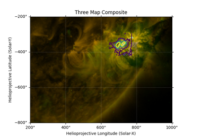
- draw_contours(levels, axes=None, *, fill=False, **contour_args)[source]#
Draw contours of the data.
- Parameters:
levels (
Quantity) – A list of numbers indicating the contours to draw. These are given as a percentage of the maximum value of the map data, or in units equivalent to theunitattribute.axes (
matplotlib.axes.Axes) – The axes on which to plot the contours. Defaults to the current axes.fill (
bool, optional) – Determines the style of the contours: - IfFalse(default), contours are drawn as lines usingcontour(). - IfTrue, contours are drawn as filled regions usingcontourf().
- Returns:
cs (
list) – TheQuadContourSetobject, after it has been added toaxes.
Notes
Extra keyword arguments to this function are passed through to the corresponding matplotlib method.
- draw_extent(*, axes=None, **kwargs)[source]#
Draw the extent of the map onto a given axes.
- Parameters:
axes (
matplotlib.axes.Axes, optional) – The axes to plot the extent on, or “None” to use current axes.- Returns:
- draw_grid(
- axes=None,
- grid_spacing=<Quantity 15. deg>,
- annotate=True,
- system='stonyhurst',
- **kwargs,
Draws a coordinate overlay on the plot in the Heliographic Stonyhurst coordinate system.
To overlay other coordinate systems see the WCSAxes Documentation
- Parameters:
axes (
axesorNone) – Axes to plot limb on, orNoneto use current axes.grid_spacing (
Quantity) – Spacing for longitude and latitude grid, if length two it specifies (lon, lat) spacing.annotate (
bool) – PassingFalsedisables the axes labels and the ticks on the top and right axes.system (str) – Coordinate system for the grid. Must be ‘stonyhurst’ or ‘carrington’.
kwargs – Additional keyword arguments are passed to
wcsaxes_heliographic_overlay.
- Returns:
overlay (
CoordinatesMap) – The wcsaxes coordinate overlay instance.
Notes
Keyword arguments are passed onto the
sunpy.visualization.wcsaxes_compat.wcsaxes_heliographic_overlayfunction.
- draw_limb(axes=None, *, resolution=1000, **kwargs)[source]#
Draws the solar limb as seen by the map’s observer.
The limb is a circle for only the simplest plots. If the coordinate frame of the limb is different from the coordinate frame of the plot axes, not only may the limb not be a true circle, a portion of the limb may be hidden from the observer. In that case, the circle is divided into visible and hidden segments, represented by solid and dotted lines, respectively.
- Parameters:
- Returns:
Notes
Keyword arguments are passed onto the patches.
If the limb is a true circle,
visiblewill instead beCircleandhiddenwill beNone. If there are no visible points (e.g., on a synoptic map any limb is fully) visiblehiddenwill beNone.To avoid triggering Matplotlib auto-scaling, these patches are added as artists instead of patches. One consequence is that the plot legend is not populated automatically when the limb is specified with a text label. See Compose custom legends in the Matplotlib documentation for examples of creating a custom legend.
- draw_quadrangle(
- bottom_left,
- *,
- width=None,
- height=None,
- axes=None,
- top_right=None,
- **kwargs,
Draw a quadrangle defined in world coordinates on the plot using Astropy’s
Quadrangle.This draws a quadrangle that has corners at
(bottom_left, top_right), and has sides aligned with the coordinate axes of the frame ofbottom_left, which may be different from the coordinate axes of the map.If
widthandheightare specified, they are respectively added to the longitude and latitude of thebottom_leftcoordinate to calculate atop_rightcoordinate.- Parameters:
bottom_left (
SkyCoordorQuantity) – The bottom-left coordinate of the rectangle. If aSkyCoordit can have shape(2,)and simultaneously definetop_right. If specifying pixel coordinates it must be given as anQuantityobject with pixel units (e.g.,pix).top_right (
SkyCoordorQuantity, optional) – The top-right coordinate of the quadrangle. Iftop_rightis specifiedwidthandheightmust be omitted.width (
astropy.units.Quantity, optional) – The width of the quadrangle. Required iftop_rightis omitted.height (
astropy.units.Quantity) – The height of the quadrangle. Required iftop_rightis omitted.axes (
matplotlib.axes.Axes) – The axes on which to plot the quadrangle. Defaults to the current axes.
- Returns:
quad (
Quadrangle) – The added patch.
Notes
Extra keyword arguments to this function are passed through to the
Quadrangleinstance.Examples
- find_contours(level, method='contourpy', **kwargs)[source]#
Returns coordinates of the contours for a given level value.
For details of the contouring algorithm, see
contourpy.contour_generator()orskimage.measure.find_contours().- Parameters:
level (float, astropy.units.Quantity) – Value along which to find contours in the array. If the map unit attribute is not
None, this must be aQuantitywith units equivalent to the map data units.method ({‘contourpy’, ‘skimage’}) – Determines which contouring method is used and should be specified as either ‘contourpy’ or ‘skimage’. Defaults to ‘contourpy’.
kwargs – Additional keyword arguments passed to either
contourpy.contour_generator()orskimage.measure.find_contours(), depending on the value of themethodargument.
- Returns:
contours (list of (n,2)
SkyCoord) – Coordinates of each contour.
Examples
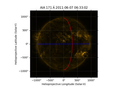
>>> import astropy.units as u
>>> import sunpy.map
>>> import sunpy.data.sample
>>> aia = sunpy.map.Map(sunpy.data.sample.AIA_171_IMAGE)
>>> contours = aia.find_contours(50000 * u.DN, method='contourpy')
>>> contours[0]
<SkyCoord (Helioprojective: obstime=2011-06-07T06:33:02.880, rsun=696000.0 km, observer=<HeliographicStonyhurst Coordinate (obstime=2011-06-07T06:33:02.880, rsun=696000.0 km): (lon, lat, radius) in (deg, deg, m)
    (-0.00406429, 0.04787238, 1.51846026e+11)>): (Tx, Ty) in arcsec
    [(713.14112796, -361.95311455), (714.76598031, -363.53013567),
     (717.17229147, -362.06880784), (717.27714042, -361.9631112 ),
     (718.43620686, -359.56313541), (718.8672722 , -357.1614    ),
     (719.58811599, -356.68119768), (721.29217122, -354.76448374),
     (722.00110323, -352.46446792), (722.08933899, -352.36363319),
     (722.00223989, -351.99536019), (721.67724425, -352.36263712),
     (719.59798458, -352.60839064), (717.19243987, -353.75348121),
     (715.8820808 , -354.75140718), (714.78652558, -355.05102034),
     (712.68209174, -357.14645009), (712.68639008, -359.54923801),
     (713.14112796, -361.95311455)]>
- classmethod is_datasource_for(data, header, **kwargs)[source]#
Determines if header corresponds to a HXI image.
- max(*args, **kwargs)[source]#
Calculate the maximum value of the data array, ignoring NaNs.
This method does preserve dask arrays.
- mean(*args, **kwargs)[source]#
Calculate the mean of the data array, ignoring NaNs.
This method does preserve dask arrays.
- min(*args, **kwargs)[source]#
Calculate the minimum value of the data array, ignoring NaNs.
This method does preserve dask arrays.
- peek(draw_limb=False, draw_grid=False, colorbar=True, **matplot_args)[source]#
Displays a graphical overview of the data in this object for user evaluation. For the creation of plots, users should instead use the
plotmethod and Matplotlib’s pyplot framework.- Parameters:
draw_limb (bool) – Whether the solar limb should be plotted.
draw_grid (bool or
Quantity) – Whether solar meridians and parallels are plotted. IfQuantitythen sets degree difference between parallels and meridians.colorbar (bool) – Whether to display a colorbar next to the plot.
**matplot_args (dict) – Matplotlib Any additional imshow arguments that should be used when plotting.
- pixel_to_world(x, y)[source]#
Convert a pixel coordinate to a data (world) coordinate.
- Parameters:
- Returns:
coord (
astropy.coordinates.SkyCoord) – A coordinate object representing the output coordinate.
- plot(
- *,
- annotate=True,
- axes=None,
- title=True,
- autoalign=True,
- clip_interval=None,
- **imshow_kwargs,
Plots the map using matplotlib.
By default, the map’s pixels will be drawn in an coordinate-aware fashion, even when the plot axes are a different projection or a different coordinate frame. See the
autoalignkeyword and the notes below.- Parameters:
annotate (
bool, optional) – IfTrue, the data is plotted at its natural scale; with title and axis labels.axes (
Axesor None) – If provided the image will be plotted on the given axes. Else the current Matplotlib axes will be used.title (
str,bool, optional) – The plot title. IfTrue, uses the default title for this map.clip_interval (two-element
Quantity, optional) – If provided, the data will be clipped to the percentile interval bounded by the two numbers.autoalign (
boolorstr, optional) – If other thanFalse, the plotting accounts for any difference between the WCS of the map and the WCS of theWCSAxesaxes (e.g., a difference in rotation angle). The options are:"mesh", which draws a mesh of the individual map pixels"image", which draws the map as a single (warped) imageTrue, which automatically determines whether to use"mesh"or"image"
**imshow_kwargs (
dict) – Any additional arguments are passed toimshow()orpcolormesh().
Examples
>>> # Simple Plot with color bar
>>> aia.plot()
>>> plt.colorbar()
>>> # Add a limb line and grid
>>> aia.plot()
>>> aia.draw_limb()
>>> aia.draw_grid()
Notes
The
autoalignfunctionality can be intensive to render. If the plot is to be interactive, the alternative approach of preprocessing the map to match the intended axes (e.g., through rotation or reprojection) will result in better plotting performance.The
autoalign='image'approach is usually faster than theautoalign='mesh'approach, but is not as reliable, depending on the specifics of the map. If parts of the map cannot be plotted, a warning is emitted. If the entire map cannot be plotted, an error is raised.When combining
autoalignfunctionality withHelioprojectivecoordinates, portions of the map that are beyond the solar disk may not appear. To preserve the off-disk parts of the map, using theSphericalScreencontext manager may be appropriate.
- quicklook()[source]#
Display a quicklook summary of the Map instance using the default web browser.
Notes
The image colormap uses histogram equalization.
Clicking on the image to switch between pixel space and coordinate space requires Javascript support to be enabled in the web browser.
Examples
>>> from sunpy.map import Map
>>> import sunpy.data.sample
>>> smap = Map(sunpy.data.sample.AIA_171_IMAGE)
>>> smap.quicklook()
(which will open the following content in the default web browser)
<sunpy.map.sources.sdo.AIAMap object at 0x7d02502a74d0>
Observatory SDO Instrument AIA 3 Detector AIA Measurement 171.0 Angstrom Wavelength 171.0 Angstrom Observation Date 2011-06-07 06:33:02 Exposure Time 0.234256 s Dimension [1024. 1024.] pix Coordinate System helioprojective Scale [2.402792 2.402792] arcsec / pix Reference Pixel [511.5 511.5] pix Reference Coord [3.22309951 1.38578135] arcsec Image colormap uses histogram equalization
Click on the image to toggle between units

- reproject_to(
- target_wcs,
- *,
- algorithm='interpolation',
- return_footprint=False,
- auto_extent=None,
- preserve_date_obs=False,
- **reproject_args,
Reproject the map to a different world coordinate system (WCS)
Additional keyword arguments are passed through to the reprojection function.
This method does not preserve dask arrays.
- Parameters:
target_wcs (
dictorWCS) – The destination FITS WCS header or WCS instancealgorithm (
str) – One of the supportedreprojectalgorithms (see below)return_footprint (
bool) – IfTrue, the footprint is returned in addition to the new map. Defaults toFalse.auto_extent (
"all","edges","corners", orNone) – IfNone, the extent of the reprojected map comes from the target WCS. If notNone, the extent of the reprojected map is automatically determined by ensuring that all of the pixels, just the edges, or just the corners of this map are in the contained within the extent. Compared to the target WCS, the extent will be shifted/expanded/cropped by an integer number of pixels. Defaults toNone.preserve_date_obs (
bool) – IfTrue, the observation time of the reprojected map is set to the observation time of the original map instead of the observation time defined in the target WCS. This does not affect the reprojection itself, which instead depends on the reference times of the two coordinate frames. Defaults toFalse.
- Returns:
outmap (
GenericMap) – The reprojected mapfootprint (
ndarray) – Footprint of the input arary in the output array. Values of 0 indicate no coverage or valid values in the input image, while values of 1 indicate valid values. Intermediate values indicate partial coverage. Only returned ifreturn_footprintisTrue.
Notes
The reprojected map does not preserve any metadata beyond the WCS-associated metadata.
The supported
reprojectalgorithms are:‘interpolation’ for
reproject_interp()‘adaptive’ for
reproject_adaptive()‘exact’ for
reproject_exact()
See the respective documentation for these functions for additional keyword arguments that are allowed.
Of the options for the automatic determination of the reprojected extent, both
"edges"and"corners"will perform the calculation faster than"all", but at the risk of potentially not including the entire reprojected map.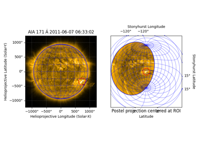
Reprojecting to a Map Projection with a Custom Origin
Reprojecting to a Map Projection with a Custom Origin
Reprojecting a Helioprojective Map to Helioprojective Radial
Reprojecting a Helioprojective Map to Helioprojective Radial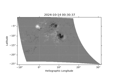
Downloading and Reprojecting a Solar Orbiter PHI/HRT Magnetogram
Downloading and Reprojecting a Solar Orbiter PHI/HRT Magnetogram
Creating a time-distance plot from a sequence of maps
Creating a time-distance plot from a sequence of maps
- resample(dimensions, method='linear')[source]#
Resample to new dimension sizes.
Uses the same parameters and creates the same coordinate lookup points as IDL’’s congrid routine, which apparently originally came from a VAX/VMS routine of the same name.
This method does not preserve dask arrays.
- Parameters:
dimensions (
Quantity) – Output pixel dimensions. The first argument corresponds to the ‘x’ axis and the second argument corresponds to the ‘y’ axis.method (str) –
- Method to use for resampling interpolation.
'nearest'and'linear'- Use n x 1-D interpolations usingscipy.interpolate.interp1d.'spline'- Uses piecewise polynomials (splines) for mapping the input array to new coordinates by interpolation usingscipy.ndimage.map_coordinates.
- Returns:
out (
GenericMapor subclass) – Resampled map
References
- rotate(
- angle=None,
- rmatrix=None,
- order=3,
- scale=1.0,
- recenter=False,
- missing=nan,
- *,
- method='scipy',
- clip=True,
Returns a new rotated and rescaled map.
Specify either a rotation angle or a rotation matrix, but not both. If neither an angle or a rotation matrix are specified, the map will be rotated by the rotation information in the metadata, which should derotate the map so that the pixel axes are aligned with world-coordinate axes.
This method does not preserve dask arrays.
- Parameters:
angle (
Quantity) – The angle (degrees) to rotate counterclockwise.rmatrix (array-like) – 2x2 linear transformation rotation matrix.
order (int) – Interpolation order to be used. The precise meaning depends on the rotation method specified by
method. Default: 3scale (float) – A scale factor for the image, default is no scaling
recenter (bool) – If
True, position the reference coordinate at the center of the new map Default:Falsemissing (float) – The value to use for pixels in the output map that are beyond the extent of the input map. Default:
numpy.nanmethod ({
'scipy','scikit-image','opencv'}, optional) – Rotation function to use. Defaults to'scipy'.clip (
bool, optional) – IfTrue, clips the pixel values of the output image to the range of the input image (including the value ofmissing, if used). Defaults toTrue.
- Returns:
out (
GenericMapor subclass) – A new Map instance containing the rotated and rescaled data of the original map.
See also
sunpy.image.transform.affine_transformThe routine this method calls for the rotation.
Notes
The rotation information in the metadata of the new map is modified appropriately from that of the original map to account for the applied rotation. It will solely be in the form of a PCi_j matrix, even if the original map used the CROTA2 keyword or a CDi_j matrix.
If the map does not already contain pixels with
numpy.nanvalues, settingmissingto an appropriate number for the data (e.g., zero) will reduce the computation time.For each NaN pixel in the input image, one or more pixels in the output image will be set to NaN, with the size of the pixel region affected depending on the interpolation order. All currently implemented rotation methods require a convolution step to handle image NaNs. This convolution normally uses
scipy.signal.convolve2d(), but if OpenCV is installed, the faster cv2.filter2D() is used instead.See
sunpy.image.transform.affine_transform()for details on each of the rotation functions.
- save(filepath, filetype='auto', **kwargs)[source]#
Save a map to a file.
- Parameters:
filepath (
str) – Location to save the file to. Iffilepathends with “.asdf” andfiletype="auto", an ASDF file will be created.filetype (
str, optional) – The file format to save the map in. Defaults to"auto"which infers the format from the file extension. Supported formats include FITS, JP2, and ASDF.hdu_type (
ExtensionHDUinstance or class, optional) – For FITS files, this specifies the type of HDU to write. By default, the map is saved in the primary HDU. If an HDU type or instance is provided, the map data and header will be written to that HDU. For example,astropy.io.fits.CompImageHDUcan be used to compress the map.kwargs – Any additional keyword arguments are passed to
write_fileorasdf.AsdfFile.write_to.
Notes
Saving with the jp2 extension will write a modified version of the given data casted to uint8 values in order to support the JPEG2000 format.
Saving with the
.asdfextension will save the map as an ASDF file, storing the map’s attributes under the key'sunpymap'in the ASDF tree.Examples
>>> from astropy.io.fits import CompImageHDU
>>> from sunpy.map import Map
>>> import sunpy.data.sample
>>> aia_map = Map(sunpy.data.sample.AIA_171_IMAGE)
>>> aia_map.save("aia171.fits", hdu_type=CompImageHDU)
>>> aia_map.save("aia171.asdf")
- shift_reference_coord(axis1, axis2)[source]#
Returns a map shifted by a specified amount to, for example, correct for a bad map location. These values are applied directly to the
reference_coordinate. To check how much the reference coordinate has been modified, seesunpy.map.GenericMap.meta.modified_items['CRVAL1']andsunpy.map.GenericMap.meta.modified_items['CRVAL2'].- Parameters:
- Returns:
out (
GenericMapor subclass) – A new shifted Map.
- std(*args, **kwargs)[source]#
Calculate the standard deviation of the data array, ignoring NaNs.
This method does preserve dask arrays.
- submap(bottom_left, *, top_right=None, width=None, height=None)[source]#
Returns a submap defined by a rectangle.
Any pixels which have at least part of their area inside the rectangle are returned. If the rectangle is defined in world coordinates, the smallest array which contains all four corners of the rectangle as defined in world coordinates is returned.
This method does preserve dask arrays.
- Parameters:
bottom_left (
astropy.units.QuantityorSkyCoord) – The bottom-left coordinate of the rectangle. If aSkyCoordit can have shape(2,)and simultaneously definetop_right. If specifying pixel coordinates it must be given as anQuantityobject with units of pixels.top_right (
astropy.units.QuantityorSkyCoord, optional) – The top-right coordinate of the rectangle. Iftop_rightis specifiedwidthandheightmust be omitted.width (
astropy.units.Quantity, optional) – The width of the rectangle. Required iftop_rightis omitted.height (
astropy.units.Quantity) – The height of the rectangle. Required iftop_rightis omitted.
- Returns:
out (
GenericMapor subclass) – A new map instance is returned representing to specified sub-region.
Notes
When specifying pixel coordinates, they are specified in Cartesian order not in numpy order. So, for example, the
bottom_left=argument should be[left, bottom].Examples
>>> import astropy.units as u
>>> from astropy.coordinates import SkyCoord
>>> import sunpy.map
>>> import sunpy.data.sample
>>> aia = sunpy.map.Map(sunpy.data.sample.AIA_171_IMAGE)
>>> bl = SkyCoord(-300*u.arcsec, -300*u.arcsec, frame=aia.coordinate_frame)
>>> tr = SkyCoord(500*u.arcsec, 500*u.arcsec, frame=aia.coordinate_frame)
>>> aia.submap(bl, top_right=tr)
<sunpy.map.sources.sdo.AIAMap object at ...>
SunPy Map
---------
Observatory:         SDO
Instrument:          AIA 3
Detector:            AIA
Measurement:         171.0 Angstrom
Wavelength:          171.0 Angstrom
Observation Date:    2011-06-07 06:33:02
Exposure Time:       0.234256 s
Dimension:           [335. 335.] pix
Coordinate System:   helioprojective
Scale:               [2.402792 2.402792] arcsec / pix
Reference Pixel:     [126.5 125.5] pix
Reference Coord:     [3.22309951 1.38578135] arcsec
...
>>> aia.submap([0,0]*u.pixel, top_right=[5,5]*u.pixel)
<sunpy.map.sources.sdo.AIAMap object at ...>
SunPy Map
---------
Observatory:         SDO
Instrument:          AIA 3
Detector:            AIA
Measurement:         171.0 Angstrom
Wavelength:          171.0 Angstrom
Observation Date:    2011-06-07 06:33:02
Exposure Time:       0.234256 s
Dimension:           [6. 6.] pix
Coordinate System:   helioprojective
Scale:               [2.402792 2.402792] arcsec / pix
Reference Pixel:     [511.5 511.5] pix
Reference Coord:     [3.22309951 1.38578135] arcsec
...
>>> width = 10 * u.arcsec
>>> height = 10 * u.arcsec
>>> aia.submap(bl, width=width, height=height)
<sunpy.map.sources.sdo.AIAMap object at ...>
SunPy Map
---------
Observatory:         SDO
Instrument:          AIA 3
Detector:            AIA
Measurement:         171.0 Angstrom
Wavelength:          171.0 Angstrom
Observation Date:    2011-06-07 06:33:02
Exposure Time:       0.234256 s
Dimension:           [5. 5.] pix
Coordinate System:   helioprojective
Scale:               [2.402792 2.402792] arcsec / pix
Reference Pixel:     [125.5 125.5] pix
Reference Coord:     [3.22309951 1.38578135] arcsec
...
>>> bottom_left_vector = SkyCoord([0, 10]  * u.deg, [0, 10] * u.deg, frame='heliographic_stonyhurst')
>>> aia.submap(bottom_left_vector)
<sunpy.map.sources.sdo.AIAMap object at ...>
SunPy Map
---------
Observatory:         SDO
Instrument:          AIA 3
Detector:            AIA
Measurement:         171.0 Angstrom
Wavelength:          171.0 Angstrom
Observation Date:    2011-06-07 06:33:02
Exposure Time:       0.234256 s
Dimension:           [70. 69.] pix
Coordinate System:   helioprojective
Scale:               [2.402792 2.402792] arcsec / pix
Reference Pixel:     [1.5 0.5] pix
Reference Coord:     [3.22309951 1.38578135] arcsec
...
- superpixel(
- dimensions,
- offset=<Quantity [0.,
- 0.] pix>,
- func=<function sum>,
- conservative_mask=False,
Returns a new map consisting of superpixels formed by applying ‘func’ to the original map data.
This method does preserve dask arrays.
- Parameters:
dimensions (tuple) – One superpixel in the new map is equal to (dimension[0], dimension[1]) pixels of the original map. The first argument corresponds to the ‘x’ axis and the second argument corresponds to the ‘y’ axis. If non-integer values are provided, they are rounded using
int.offset (tuple) – Offset from (0,0) in original map pixels used to calculate where the data used to make the resulting superpixel map starts. If non-integer value are provided, they are rounded using
int.func – Function applied to the original data. The function ‘func’ must take a numpy array as its first argument, and support the axis keyword with the meaning of a numpy axis keyword (see the description of
sumfor an example.) The default value of ‘func’ issum; using this causes superpixel to sum over (dimension[0], dimension[1]) pixels of the original map.conservative_mask (bool, optional) – If
True, a superpixel is masked if any of its constituent pixels are masked. IfFalse, a superpixel is masked only if all of its constituent pixels are masked. Default isFalse.
- Returns:
out (
GenericMapor subclass) – A new Map which has superpixels of the required size.
- world_to_pixel(coordinate)[source]#
Convert a world (data) coordinate to a pixel coordinate.
- Parameters:
coordinate (
SkyCoordorBaseCoordinateFrame) – The coordinate object to convert to pixel coordinates.- Returns: