Note
Go to the end to download the full example code.
Drawing the AIA limb on a STEREO EUVI image#
In this example we use a STEREO-B and an SDO image to demonstrate how to overplot the limb as seen by AIA on an EUVI-B image. Then we overplot the AIA coordinate grid on the STEREO image.
import matplotlib.pyplot as plt

import astropy.units as u
from astropy.coordinates import SkyCoord

import sunpy.coordinates.wcs_utils
import sunpy.map
from sunpy.data.sample import AIA_193_JUN2012, STEREO_B_195_JUN2012
Let’s create a dictionary with the two maps, which we crop to full disk.
maps = {m.detector: m.submap(SkyCoord([-1100, 1100], [-1100, 1100],
                                      unit=u.arcsec, frame=m.coordinate_frame))
        for m in sunpy.map.Map([AIA_193_JUN2012, STEREO_B_195_JUN2012])}
maps['AIA'].plot_settings['vmin'] = 0  # set the minimum plotted pixel value
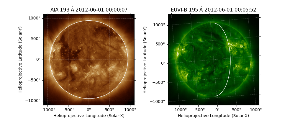
Now, let’s plot both maps, and we draw the limb as seen by AIA onto the EUVI image. We remove the part of the limb that is hidden because it is on the far side of the Sun from STEREO’s point of view.
fig = plt.figure(figsize=(10, 4))
ax1 = fig.add_subplot(121, projection=maps['AIA'])
maps['AIA'].plot(axes=ax1)
maps['AIA'].draw_limb(axes=ax1)

ax2 = fig.add_subplot(122, projection=maps['EUVI'])
maps['EUVI'].plot(axes=ax2)
visible, hidden = maps['AIA'].draw_limb(axes=ax2)
hidden.remove()
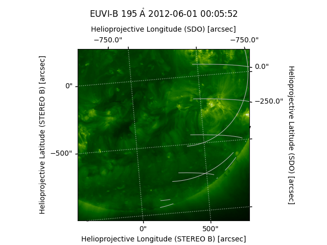
Let’s plot the helioprojective coordinate grid as seen by SDO on the STEREO image in a cropped view. Note that only those grid lines that intersect the edge of the plot will have corresponding ticks and tick labels.
fig = plt.figure()
ax = fig.add_subplot(projection=maps['EUVI'])

maps['EUVI'].plot(axes=ax)

# Crop the view using pixel coordinates
ax.set_xlim(500, 1300)
ax.set_ylim(100, 900)

# Shrink the plot slightly and move the title up to make room for new labels.
ax.set_position([0.1, 0.1, 0.8, 0.7])
ax.set_title(ax.get_title(), pad=45)

# Change the default grid labels and line properties.
stereo_x, stereo_y = ax.coords
stereo_x.set_axislabel("Helioprojective Longitude (STEREO B) [arcsec]")
stereo_y.set_axislabel("Helioprojective Latitude (STEREO B) [arcsec]")
ax.coords.grid(color='white', linewidth=1)

# Add a new coordinate overlay in the SDO frame.
overlay = ax.get_coords_overlay(maps['AIA'].coordinate_frame)
overlay.grid()

# Configure the grid:
x, y = overlay

# Wrap the longitude at 180 deg rather than the default 360.
x.set_coord_type('longitude', 180*u.deg)

# Set the tick spacing
x.set_ticks(spacing=250*u.arcsec)
y.set_ticks(spacing=250*u.arcsec)

# Set the ticks to be on the top and left axes.
x.set_ticks_position('tr')
y.set_ticks_position('tr')

# Change the defaults to arcseconds
x.set_major_formatter('s.s')
y.set_major_formatter('s.s')

# Add axes labels
x.set_axislabel("Helioprojective Longitude (SDO) [arcsec]")
y.set_axislabel("Helioprojective Latitude (SDO) [arcsec]")

plt.show()
Total running time of the script: (0 minutes 1.559 seconds)