Blending maps using mplcairo

This example shows how to blend two maps using mplcairo.

matplotlib by itself provides only alpha-based transparency for superimposing one image onto another, which can be restrictive when trying to create visually appealing composite images. mplcairo is an enhancement for matplotlib that provides support for cairo’s compositing operators, which include a wide range of blend modes for image overlays.

Note

This example requires mplcairo to be installed. Installation via pip will work in most cases, but you may need to refer to OS-specific installation notes.

We need to tell matplotlib to use a backend from mplcairo. The backend formally needs to be set prior to importing matplotlib.pyplot. The mplcairo.qt GUI backend should work on Linux and Windows, but you will need to use something different on macOS or Jupyter (see mplcairo’s usage notes).

import matplotlib

if matplotlib.get_backend() == "agg":
    # This is the non-GUI backend for when building the documentation
    matplotlib.use("module://mplcairo.base")
else:
    # This is a GUI backend that you would normally use
    matplotlib.use("module://mplcairo.qt")

We can now import everything else.

import matplotlib.pyplot as plt
from mplcairo import operator_t

import astropy.units as u

import sunpy.data.sample
import sunpy.map
from sunpy.coordinates import SphericalScreen

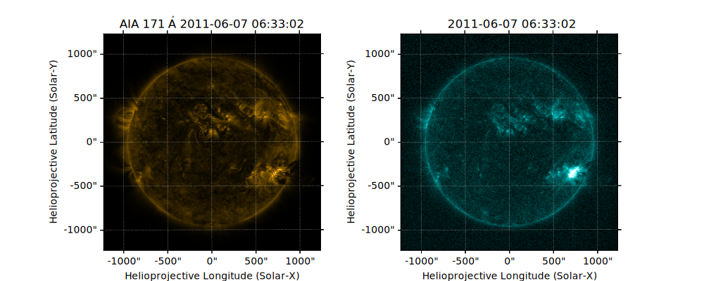
Let’s load two maps for blending. We reproject the second map to the coordinate frame of the first map for proper compositing, taking care to use the SphericalScreen context manager in order to preserve off-disk data.

a171 = sunpy.map.Map(sunpy.data.sample.AIA_171_IMAGE)
a131 = sunpy.map.Map(sunpy.data.sample.AIA_131_IMAGE)
with SphericalScreen(a171.observer_coordinate):
    a131 = a131.reproject_to(a171.wcs)

Let’s first plot the two maps individually.

fig1 = plt.figure(figsize=(10, 4))
ax1 = fig1.add_subplot(121, projection=a171)
ax2 = fig1.add_subplot(122, projection=a131)

a171.plot(axes=ax1, clip_interval=(1, 99.9995)*u.percent)
a131.plot(axes=ax2, clip_interval=(1, 99.95)*u.percent)

<matplotlib.image.AxesImage object at 0x7ff094ab9af0>

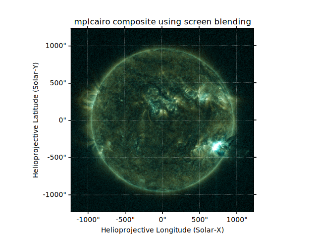
We now plot the two maps on the same axes. If the plot were rendered at this point, the second map would completely obscure the first map. We save the matplotlib artist returned when plotting the second map (im131) for future use.

fig2 = plt.figure()
ax = fig2.add_subplot(projection=a171)

a171.plot(axes=ax, clip_interval=(1, 99.9995)*u.percent)
im131 = a131.plot(axes=ax, clip_interval=(1, 99.95)*u.percent)

We invoke the mplcairo operator for the screen blend mode to modify the artist for the second map. The second map will now be composited onto the first map using that blend mode.

operator_t.SCREEN.patch_artist(im131)

Finally, we set the title and render the plot.

ax.set_title('mplcairo composite using screen blending')
plt.show()