Note
Go to the end to download the full example code.
Tracing Coronal Loops and Extracting Intensities#
This example traces out the coronal loops in a FITS image
using occult2 and then extracts the intensity
along one traced loop.
In this example we will use the settings and the data from Markus Aschwanden’s tutorial
on his IDL implementation of the OCCULT2 algorithm, which can be found
here.
import matplotlib.pyplot as plt
import numpy as np

from astropy import units as u
from astropy.io import fits

import sunpy.map

import sunkit_image.trace as trace
We will be using astropy.io.fits.open to read the FITS file used in the tutorial
and read in the header and data information.
with fits.open("http://data.sunpy.org/sunkit-image/trace_1998-05-19T22:21:43.000_171_1024.fits") as hdul:
    # We can now make this into a `sunpy.map.GenericMap`.
    trace_map = sunpy.map.Map(hdul[0].data, hdul[0].header)
    # We need to set the colormap manually to match the IDL tutorial as close as possible.
    trace_map.plot_settings["cmap"] = "goes-rsuvi304"
Now the loop tracing will begin. We will use the same set of parameters as in the IDL tutorial.
The lowpass filter boxcar filter size nsm1 is taken to be 3.
The minimum radius of curvature at any point in the loop rmin is 30 pixels.
The length of the smallest loop to be detected lmin is 25 pixels.
The maximum number of structures to be examined nstruc is 1000.
The number of extra points in the loop below noise level to terminate a loop tracing ngap is 0.
The base flux and median flux ratio qthresh1 is 0.0.
The noise threshold in the image with respect to median flux qthresh2 is 3.0 .
For the meaning of these parameters please consult the OCCULT2 article.
loops = trace.occult2(trace_map, nsm1=3, rmin=30, lmin=25, nstruc=1000, ngap=0, qthresh1=0.0, qthresh2=3.0)
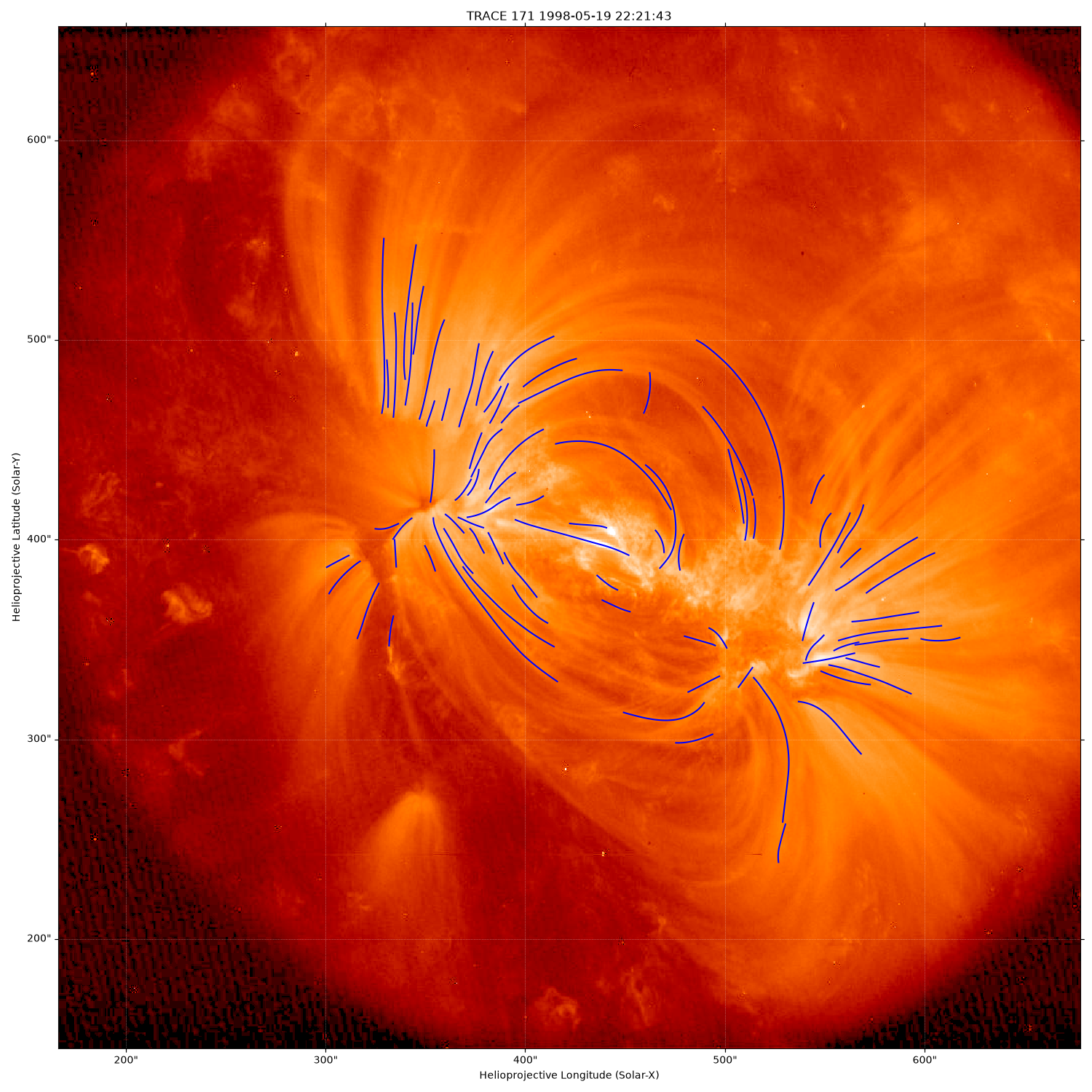
occult2 returns a list, each element of which is a detected loop.
Each detected loop is stored as a list of x positions in image pixels, and a list of y
positions in image pixels, of the pixels traced out by OCCULT2.
Now plot all the detected loops on the original image, we convert the image pixels to
to world coordinates to be plotted on the map.
fig = plt.figure(figsize=(15, 15))

ax = fig.add_subplot(projection=trace_map)
trace_map.plot(axes=ax, clip_interval=(1, 99.99) * u.percent)
# We can now plot each loop in the list of loops.
# We plot these in world coordinates, converting them through the `pixel_to_world`
# functionality which converts the pixel coordinates to coordinates (in arcsec) on the ``trace_map``.
for loop in loops:
    loop = np.array(loop)  # convert to array as easier to index ``x`` and ``y`` coordinates
    coord_loops = trace_map.pixel_to_world(loop[:, 0] * u.pixel, loop[:, 1] * u.pixel)
    ax.plot_coord(coord_loops, color="b")

fig.tight_layout()
INFO: Missing metadata for solar radius: assuming the standard radius of the photosphere. [sunpy.map.mapbase]
/home/docs/checkouts/readthedocs.org/user_builds/sunkit-image/conda/latest/lib/python3.12/site-packages/sunpy/map/mapbase.py:671: SunpyMetadataWarning: Missing metadata for observer: assuming Earth-based observer.
For frame 'heliographic_stonyhurst' the following metadata is missing: hglt_obs,hgln_obs,dsun_obs
For frame 'heliographic_carrington' the following metadata is missing: crlt_obs,crln_obs,dsun_obs

  obs_coord = self.observer_coordinate
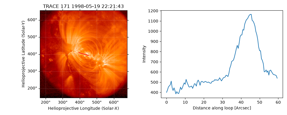
Finally, we can use the traced loops location information to extract the intensity values.
# Since we only currently get pixel locations, we need to get the word coordinates of the first loop.
first_loop = np.array(loops[0])
loop_coords = trace_map.pixel_to_world(first_loop[:, 0] * u.pixel, first_loop[:, 1] * u.pixel)

# Now we can extract the intensity along the loop
intensity = sunpy.map.sample_at_coords(trace_map, loop_coords)

# Finally, we can calculate the angular separation along the loop
angular_separation = loop_coords.separation(loop_coords[0]).to(u.arcsec)

# Plot the loop location and its intensity profile
fig = plt.figure(figsize=(10, 4))
ax = fig.add_subplot(121, projection=trace_map)
trace_map.plot(axes=ax, clip_interval=(1, 99.99) * u.percent)
ax.plot_coord(loop_coords, color="r")

ax = fig.add_subplot(122)
ax.plot(angular_separation, intensity)
ax.set_xlabel("Distance along loop [Arcsec]")
ax.set_ylabel("Intensity")

fig.tight_layout()

plt.show()
Total running time of the script: (0 minutes 22.359 seconds)