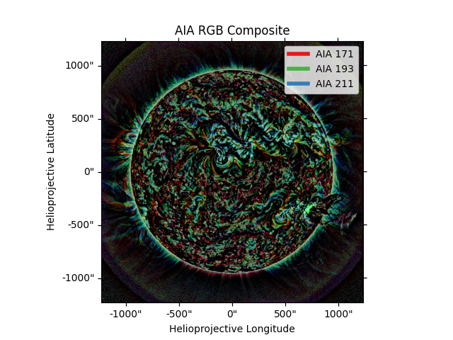
Making an RGB composite image

This example shows the process required to create an RGB composite image of three AIA images at different wavelengths. To read more about the algorithm used in this example, see this Astropy tutorial.

import matplotlib.pyplot as plt
import sunpy.data.sample
from astropy.visualization import make_lupton_rgb
from matplotlib.lines import Line2D
from sunpy.map import Map

from sunkit_image.enhance import mgn

We will use three AIA images from the sample data at the following wavelengths: 171, 193, and 211 Angstroms. The 171 image shows the quiet solar corona, 193 shows a hotter region of the corona, and 211 shows active magnetic regions in the corona.

maps = Map(sunpy.data.sample.AIA_171_IMAGE, sunpy.data.sample.AIA_193_IMAGE, sunpy.data.sample.AIA_211_IMAGE)

Files Downloaded:   0%|          | 0/1 [00:00<?, ?file/s]

AIA20110607_063307_0193_lowres.fits:   0%|          | 0.00/1.00M [00:00<?, ?B/s]


Files Downloaded: 100%|██████████| 1/1 [00:00<00:00,  1.98file/s]
Files Downloaded: 100%|██████████| 1/1 [00:00<00:00,  1.98file/s]

Files Downloaded:   0%|          | 0/1 [00:00<?, ?file/s]

AIA20110607_063302_0211_lowres.fits:   0%|          | 0.00/988k [00:00<?, ?B/s]


Files Downloaded: 100%|██████████| 1/1 [00:00<00:00,  1.89file/s]
Files Downloaded: 100%|██████████| 1/1 [00:00<00:00,  1.89file/s]

Before the images are assigned colors and combined, they need to be normalized so that features in each wavelength are visible in the combined image. We will apply multi-scale Gaussian normalization using sunkit_image.enhance.mgn to each map and then create the rgb composite. The k parameter is a scaling factor applied to the normalized image. A value of 5 produces sharper details in the transformed image. In the make_lupton_rgb function, Q is a softening parameter which we set to 0 and stretch controls the linear stretch applied to the combined image.

maps_mgn = [Map(mgn(m.data, k=5), m.meta) for m in maps]
im_rgb = make_lupton_rgb(maps_mgn[0].data, maps_mgn[1].data, maps_mgn[2].data, Q=0, stretch=1)

The output of the astropy.visualization.make_lupton_rgb algorithm is not a Map, but instead an image. So, we need to create a WCS Axes using one of original maps and manually set the label. In the first step below, we grab the Set1 qualitative colormap to apply to the custom legend lines.

cmap = plt.cm.Set1
custom_lines = [
    Line2D([0], [0], color=cmap(0), lw=4),
    Line2D([0], [0], color=cmap(2), lw=4),
    Line2D([0], [0], color=cmap(1), lw=4),
]
fig = plt.figure()
ax = fig.add_subplot(111, projection=maps[0].wcs)
im = ax.imshow(im_rgb)
lon, lat = ax.coords
lon.set_axislabel("Helioprojective Longitude")
lat.set_axislabel("Helioprojective Latitude")
ax.legend(custom_lines, ["AIA 171", "AIA 193", "AIA 211"])
ax.set_title("AIA RGB Composite")

plt.show()