Coaligning EIS to AIA

This example shows how to coalign EIS rasters to AIA images in order correct for the pointing uncertainty in EIS.

import matplotlib.pyplot as plt

import astropy.units as u
from astropy.visualization import AsinhStretch, ImageNormalize

import sunpy.map

from sunkit_image.coalignment import coalign_map

For this example, we will use a preprocessed EIS raster image of the Fe XII 195.119 Å line. This raster image was prepared using the eispac package.

eis_map = sunpy.map.Map(
    "https://github.com/sunpy/data/raw/main/sunkit-image/eis_20140108_095727.fe_12_195_119.2c-0.int.fits"
)

Next, let’s download the AIA data we will use as a reference image. We want AIA data near the beginning of the EIS raster and we’ll use the 193 Å channel of AIA as it sees plasma at approximately the same temperature as the 195.119 Å line in our EIS raster. We have stored this file on Github so we can download it directly.

aia_map = sunpy.map.Map(
    "https://github.com/sunpy/data/raw/refs/heads/main/sunkit-image/aia.lev1.193A_2014_01_08T09_57_30.84Z.image_lev1.fits"
)

Before coaligning the images, we first resample the AIA image to the same plate scale as the EIS image. This will ensure better results from our coalignment.

nx = (aia_map.scale.axis1 * aia_map.dimensions.x) / eis_map.scale.axis1
ny = (aia_map.scale.axis2 * aia_map.dimensions.y) / eis_map.scale.axis2

aia_downsampled = aia_map.resample(u.Quantity([nx, ny]))

Now we can coalign EIS and AIA using cross-correlation. By default, this function uses the “match_template” method. For details of the implementation refer to the documentation of skimage.feature.match_template.

coaligned_eis_map = coalign_map(eis_map, aia_downsampled)

INFO: Missing metadata for solar radius: assuming the standard radius of the photosphere. [sunpy.map.mapbase]
INFO: Missing metadata for solar radius: assuming the standard radius of the photosphere. [sunpy.map.mapbase]

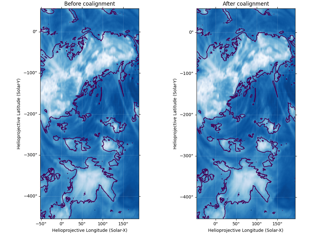
To check now effective this has been, we will plot the EIS data and overlap the bright regions from AIA before and after the coalignment.

fig = plt.figure(figsize=(10, 7.5), layout="constrained")
ax = fig.add_subplot(121, projection=eis_map)
eis_map.plot(
    axes=ax,
    title="Before coalignment",
    aspect=eis_map.scale.axis2 / eis_map.scale.axis1,
    cmap="Blues_r",
    norm=ImageNormalize(stretch=AsinhStretch()),
)
aia_map.draw_contours([800] * aia_map.unit, axes=ax)
ax = fig.add_subplot(122, projection=coaligned_eis_map, sharex=ax, sharey=ax)
coaligned_eis_map.plot(
    axes=ax,
    title="After coalignment",
    aspect=coaligned_eis_map.scale.axis2 / coaligned_eis_map.scale.axis1,
    cmap="Blues_r",
    norm=ImageNormalize(stretch=AsinhStretch()),
)
aia_map.draw_contours([800] * aia_map.unit, axes=ax)

INFO: Missing metadata for solar radius: assuming the standard radius of the photosphere. [sunpy.map.mapbase]
INFO: Missing metadata for solar radius: assuming the standard radius of the photosphere. [sunpy.map.mapbase]

<matplotlib.contour.QuadContourSet object at 0x75763da59370>

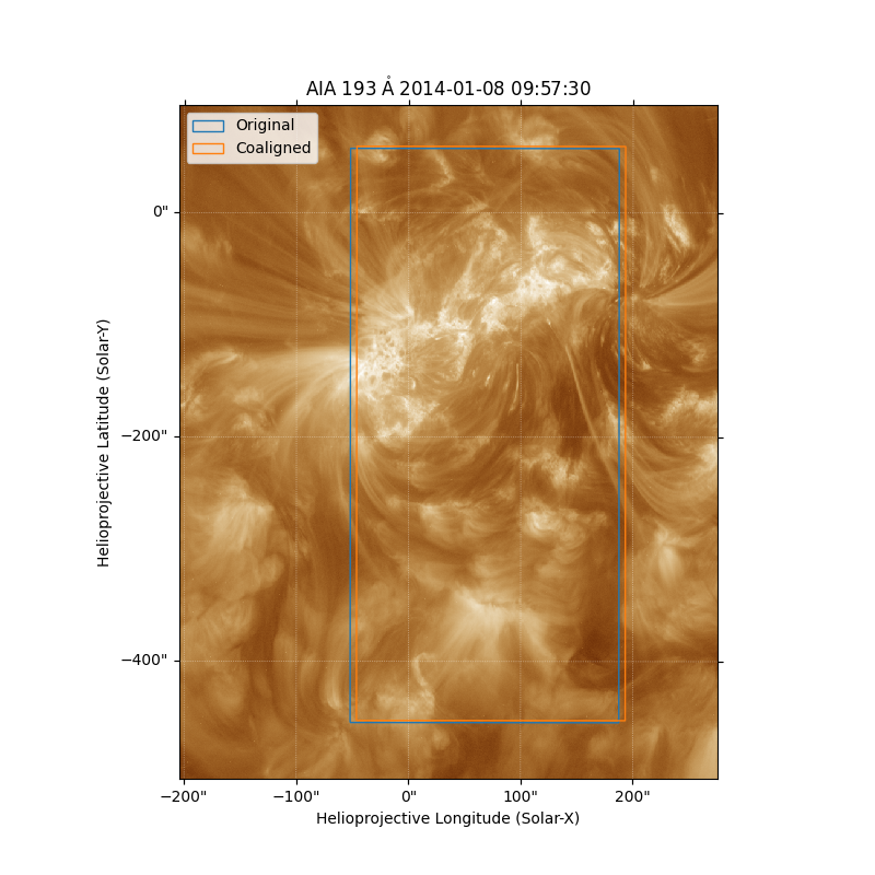
We can also visualize this shift by overlaying the extent of the two EIS maps on the AIA image we used to perform the coalignment.

fig = plt.figure(figsize=(8, 8))
ax = fig.add_subplot(projection=aia_map)
aia_map.plot(axes=ax)
eis_map.draw_extent(axes=ax, color="C0", label="Original")
coaligned_eis_map.draw_extent(axes=ax, color="C1", label="Coaligned")
ax.set_xlim(1700, 2500)
ax.set_ylim(1200, 2200)
ax.legend()

plt.show()