Combining a celestial WCS with a wavelength axis

The goal of this example is to construct a spectral-image cube of AIA images at different wavelengths.

This will showcase how to add an arbitrarily spaced wavelength dimension to a celestial WCS.

import matplotlib.pyplot as plt

import astropy.units as u

import sunpy.data.sample
import sunpy.map

from ndcube import NDCube
from ndcube.extra_coords import QuantityTableCoordinate
from ndcube.wcs.wrappers import CompoundLowLevelWCS

We will use the sample data that sunpy provides to construct a sequence of AIA image files for different wavelengths using sunpy.map.Map.

aia_files = [sunpy.data.sample.AIA_094_IMAGE,
             sunpy.data.sample.AIA_131_IMAGE,
             sunpy.data.sample.AIA_171_IMAGE,
             sunpy.data.sample.AIA_193_IMAGE,
             sunpy.data.sample.AIA_211_IMAGE,
             sunpy.data.sample.AIA_304_IMAGE,
             sunpy.data.sample.AIA_335_IMAGE,
             sunpy.data.sample.AIA_1600_IMAGE]
# `sequence=True` causes a sequence of maps to be returned, one for each image file.
sequence_of_maps = sunpy.map.Map(aia_files, sequence=True)
# Sort the maps in the sequence in order of wavelength.
sequence_of_maps.maps = list(sorted(sequence_of_maps.maps, key=lambda m: m.wavelength))

Files Downloaded:   0%|          | 0/1 [00:00<?, ?file/s]

AIA20110607_063305_0094_lowres.fits:   0%|          | 0.00/971k [00:00<?, ?B/s]


Files Downloaded: 100%|██████████| 1/1 [00:00<00:00,  2.26file/s]
Files Downloaded: 100%|██████████| 1/1 [00:00<00:00,  2.26file/s]

Files Downloaded:   0%|          | 0/1 [00:00<?, ?file/s]

AIA20110607_063301_0131_lowres.fits:   0%|          | 0.00/962k [00:00<?, ?B/s]


Files Downloaded: 100%|██████████| 1/1 [00:00<00:00,  2.34file/s]
Files Downloaded: 100%|██████████| 1/1 [00:00<00:00,  2.33file/s]

Files Downloaded:   0%|          | 0/1 [00:00<?, ?file/s]

AIA20110607_063302_0171_lowres.fits:   0%|          | 0.00/973k [00:00<?, ?B/s]


Files Downloaded: 100%|██████████| 1/1 [00:00<00:00,  2.12file/s]
Files Downloaded: 100%|██████████| 1/1 [00:00<00:00,  2.11file/s]

Files Downloaded:   0%|          | 0/1 [00:00<?, ?file/s]

AIA20110607_063307_0193_lowres.fits:   0%|          | 0.00/1.00M [00:00<?, ?B/s]


Files Downloaded: 100%|██████████| 1/1 [00:00<00:00,  1.45file/s]
Files Downloaded: 100%|██████████| 1/1 [00:00<00:00,  1.45file/s]

Files Downloaded:   0%|          | 0/1 [00:00<?, ?file/s]

AIA20110607_063302_0211_lowres.fits:   0%|          | 0.00/988k [00:00<?, ?B/s]


Files Downloaded: 100%|██████████| 1/1 [00:00<00:00,  2.13file/s]
Files Downloaded: 100%|██████████| 1/1 [00:00<00:00,  2.13file/s]

Files Downloaded:   0%|          | 0/1 [00:00<?, ?file/s]

AIA20110607_063334_0304_lowres.fits:   0%|          | 0.00/965k [00:00<?, ?B/s]


Files Downloaded: 100%|██████████| 1/1 [00:00<00:00,  2.65file/s]
Files Downloaded: 100%|██████████| 1/1 [00:00<00:00,  2.65file/s]

Files Downloaded:   0%|          | 0/1 [00:00<?, ?file/s]

AIA20110607_063303_0335_lowres.fits:   0%|          | 0.00/979k [00:00<?, ?B/s]


Files Downloaded: 100%|██████████| 1/1 [00:00<00:00,  1.97file/s]
Files Downloaded: 100%|██████████| 1/1 [00:00<00:00,  1.97file/s]

Files Downloaded:   0%|          | 0/1 [00:00<?, ?file/s]

AIA20110607_063305_1600_lowres.fits:   0%|          | 0.00/930k [00:00<?, ?B/s]


Files Downloaded: 100%|██████████| 1/1 [00:00<00:00,  2.19file/s]
Files Downloaded: 100%|██████████| 1/1 [00:00<00:00,  2.19file/s]

Using an astropy.units.Quantity of the wavelengths of the images, we can construct a 1D lookup-table WCS via QuantityTableCoordinate. This is then combined with the celestial WCS into a single 3D WCS via CompoundLowLevelWCS.

wavelengths = u.Quantity([m.wavelength for m in sequence_of_maps])
wavelengths_wcs = QuantityTableCoordinate(wavelengths, physical_types="em.wl", names="wavelength").wcs
cube_wcs = CompoundLowLevelWCS(wavelengths_wcs, sequence_of_maps[0].wcs)

Combine the new 3D WCS with the stack of AIA images using ndcube.NDCube. Note that because we set the wavelength to the first axis in the WCS (cube_wcs), the final data cube is stacked such that wavelength corresponds to the array axis which is last. This is due to the convention that WCS axis ordering is reversed compared to data array axis ordering.

my_cube = NDCube(sequence_of_maps.as_array(), wcs=cube_wcs)
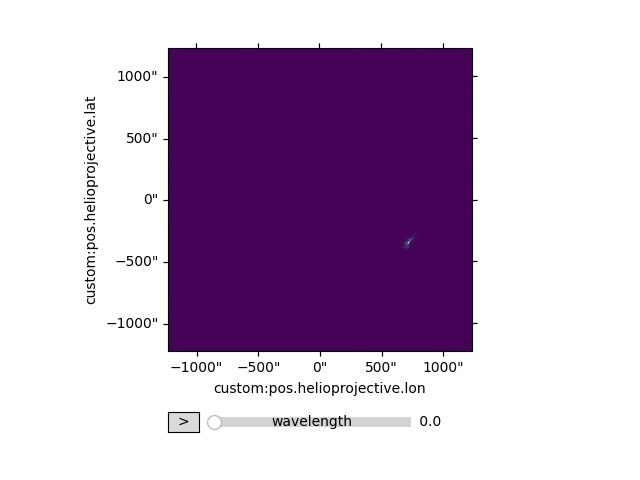
# Produce an interactive plot of the spectral-image stack.
my_cube.plot(plot_axes=['y', 'x', None])

plt.show()

/home/docs/checkouts/readthedocs.org/user_builds/ndcube/conda/latest/lib/python3.11/site-packages/astropy/units/format/utils.py:220: UnitsWarning: The unit 'Angstrom' has been deprecated in the VOUnit standard. Suggested: 0.1nm.
  warnings.warn(message, UnitsWarning)