Downloading and plotting solar modes with HMI

This example shows how to download HMI data from JSOC and make a plot of the solar modes.

import matplotlib.pyplot as plt
import numpy as np

import drms

First we will create a drms.Client, using the JSOC baseurl.

client = drms.Client()

Construct the DRMS query string: “Series[timespan][wavelength]”

qstr = "hmi.v_sht_modes[2014.06.20_00:00:00_TAI]"

# TODO: Add text here.
segname = "m6"  # 'm6', 'm18' or 'm36'

# Send request to the DRMS server
print(f"Querying keyword data...\n -> {qstr}")
result, filenames = client.query(qstr, key=["T_START", "T_STOP", "LMIN", "LMAX", "NDT"], seg=segname)
print(f" -> {len(result)} lines retrieved.")

# Use only the first line of the query result
result = result.iloc[0]
fname = f"http://jsoc.stanford.edu{filenames[segname][0]}"

# Read the data segment
print(f"Reading data from {fname}...")
a = np.genfromtxt(fname)

# For column names, see appendix of Larson & Schou (2015SoPh..290.3221L)
l = a[:, 0].astype(int)
n = a[:, 1].astype(int)
nu = a[:, 2] / 1e3
if a.shape[1] in [24, 48, 84]:
    # tan(gamma) present
    sig_offs = 5
elif a.shape[1] in [26, 50, 86]:
    # tan(gamma) not present
    sig_offs = 6
snu = a[:, sig_offs + 2] / 1e3

Querying keyword data...
 -> hmi.v_sht_modes[2014.06.20_00:00:00_TAI]
 -> 2 lines retrieved.
Reading data from http://jsoc.stanford.edu/SUM11/D608023042/S00000/m10qr.7840...

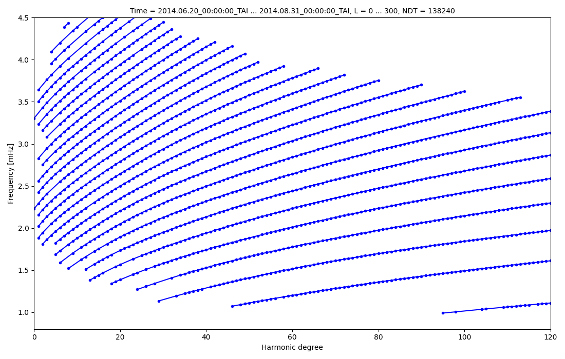
Plot the zoomed in on lower l

fig, ax = plt.subplots(1, 1, figsize=(11, 7))
ax.set_title(
    f"Time = {result.T_START} ... {result.T_STOP}, L = {result.LMIN} ... {result.LMAX}, NDT = {result.NDT}",
    fontsize="medium",
)
for ni in np.unique(n):
    idx = n == ni
    ax.plot(l[idx], nu[idx], "b.-")
ax.set_xlim(0, 120)
ax.set_ylim(0.8, 4.5)
ax.set_xlabel("Harmonic degree")
ax.set_ylabel("Frequency [mHz]")
fig.tight_layout()

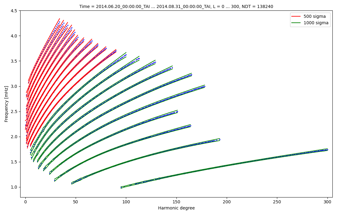
Plot the zoomed in on higher l, n <= 20, with errors

fig, ax = plt.subplots(1, 1, figsize=(11, 7))
ax.set_title(
    f"Time = {result.T_START} ... {result.T_STOP}, L = {result.LMIN} ... {result.LMAX}, NDT = {result.NDT}",
    fontsize="medium",
)
for ni in np.unique(n):
    if ni <= 20:
        idx = n == ni
        ax.plot(l[idx], nu[idx], "b.", ms=3)
        if ni < 10:
            ax.plot(l[idx], nu[idx] + 1000 * snu[idx], "g")
            ax.plot(l[idx], nu[idx] - 1000 * snu[idx], "g")
        else:
            ax.plot(l[idx], nu[idx] + 500 * snu[idx], "r")
            ax.plot(l[idx], nu[idx] - 500 * snu[idx], "r")
ax.legend(
    loc="upper right",
    handles=[
        plt.Line2D([0], [0], color="r", label="500 sigma"),
        plt.Line2D([0], [0], color="g", label="1000 sigma"),
    ],
)
ax.set_xlim(-5, 305)
ax.set_ylim(0.8, 4.5)
ax.set_xlabel("Harmonic degree")
ax.set_ylabel("Frequency [mHz]")
fig.tight_layout()

plt.show()