Searching for and plotting a WIND/WAVES spectrogram

This example demonstrates how to download and plot a WIND/WAVES spectrogram using sunpy.net.Fido and the Spectrogram class.

WAVES is the radio and plasma wave instrument on the WIND spacecraft. Its two radio receivers, RAD1 (20-1040 kHz) and RAD2 (1.075-13.825 MHz)

import matplotlib.pyplot as plt

from sunpy.net import Fido
from sunpy.net import attrs as a

from radiospectra import net  # noqa: F401
from radiospectra.spectrogram import Spectrogram

First, let’s search for some WIND/WAVES data during a known event. We will search for data on 2017-09-02 between 15:00 and 18:00.

query = Fido.search(a.Time("2017-09-02T15:00", "2017-09-02T18:00"), a.Instrument.waves)
print(query)

Results from 1 Provider:

2 Results from the WAVESClient:

       Start Time               End Time        Instrument Source Provider     Wavelength
                                                                                  kHz
----------------------- ----------------------- ---------- ------ -------- -----------------
2017-09-02 00:00:00.000 2017-09-02 23:59:59.999      WAVES   WIND     SPDF    20.0 .. 1040.0
2017-09-02 00:00:00.000 2017-09-02 23:59:59.999      WAVES   WIND     SPDF 1075.0 .. 13825.0

Now we fetch the files using sunpy.net.Fido and load them into a Spectrogram object. With no Wavelength specified, the search returns one file per receiver (RAD1 and RAD2).

waves_files = Fido.fetch(query["waves"])
waves_spec = Spectrogram(sorted(waves_files))

Files Downloaded:   0%|          | 0/2 [00:00<?, ?file/s]


wind_waves_rad2_20170902.R2: 0.00B [00:00, ?B/s]

wind_waves_rad1_20170902.R1: 0.00B [00:00, ?B/s]


wind_waves_rad2_20170902.R2: 42.5kB [00:00, 414kB/s]

wind_waves_rad1_20170902.R1: 1.02kB [00:00, 8.22kB/s]



Files Downloaded:  50%|█████     | 1/2 [00:00<00:00,  3.40file/s]

wind_waves_rad1_20170902.R1: 588kB [00:00, 3.12MB/s]


Files Downloaded: 100%|██████████| 2/2 [00:00<00:00,  5.32file/s]

We can print a string representation of the downloaded spectrograms. As the search matched both receivers, waves_spec is a list with one spectrogram per receiver. Sorting the files by name places the RAD1 (lower-frequency) spectrogram first and RAD2 (higher-frequency) second.

print(waves_spec)

[<WAVESSpectrogram WIND, WAVES, RAD1 20.0 kHz - 1040.0 kHz, 2017-09-02T00:00:00.000 to 2017-09-02T23:59:59.000>, <WAVESSpectrogram WIND, WAVES, RAD2 1075.0 kHz - 13825.0 kHz, 2017-09-02T00:00:00.000 to 2017-09-02T23:59:59.000>]

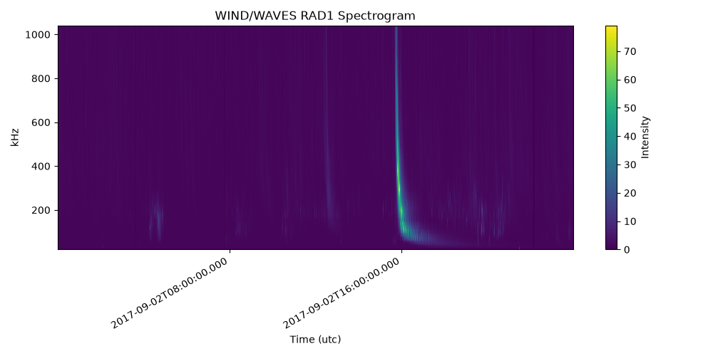
Finally, let’s plot the first spectrogram (RAD1) using matplotlib. The plot() method automatically formats the axes.

fig, ax = plt.subplots(figsize=(10, 5))
mesh = waves_spec[0].plot(axes=ax)
fig.colorbar(mesh, ax=ax, label="Intensity")
ax.set_title("WIND/WAVES RAD1 Spectrogram")
fig.tight_layout()
plt.show()