Note
Go to the end to download the full example code
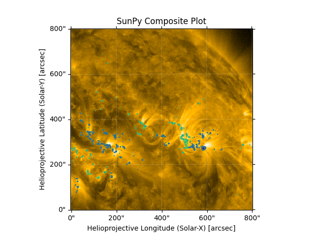
Creating a Composite map#
How to create a composite map and use it to overplot two maps to compare features.
import matplotlib.pyplot as plt

import astropy.units as u
from astropy.coordinates import SkyCoord

import sunpy.data.sample
import sunpy.map
We start with the sample data. HMI shows the line-of-sight magnetic field at the photosphere while AIA 171 images show the resulting magnetic fields filled with hot plasma above, in the corona. We want to see what coronal features overlap with regions of strong line-of-sight magnetic fields.
aia_map = sunpy.map.Map(sunpy.data.sample.AIA_171_IMAGE)
hmi_map = sunpy.map.Map(sunpy.data.sample.HMI_LOS_IMAGE)

bottom_left = [0, 0] * u.arcsec
top_right = [800, 800] * u.arcsec
aia_smap = aia_map.submap(SkyCoord(*bottom_left, frame=aia_map.coordinate_frame),
                          top_right=SkyCoord(*top_right, frame=aia_map.coordinate_frame))
hmi_smap = hmi_map.submap(SkyCoord(*bottom_left, frame=hmi_map.coordinate_frame),
                          top_right=SkyCoord(*top_right, frame=hmi_map.coordinate_frame))
Let’s create a CompositeMap which includes both maps.
comp_map = sunpy.map.Map(aia_smap, hmi_smap, composite=True)

# Let's set the contours of the HMI map, the second image in our composite map
# (therefore the index is 1), from a few hundred to a thousand Gauss which
# is the typical field associated with umbral regions of active regions.
levels = [-1000, -500, -250, 250, 500, 1000] * u.G
comp_map.set_levels(index=1, levels=levels)
Now let us look at the result. Notice that we can see the coronal structures present on the AIA image and how they correspond to the line of sight magnetic field.
fig = plt.figure()
ax = fig.add_subplot(projection=comp_map.get_map(0))
comp_map.plot(axes=ax)
plt.show()
Total running time of the script: (0 minutes 0.722 seconds)